Complex Numbers

Complex numbers are fundamental to signal processing. They provide an elegant way to represent and manipulate sinusoidal signals, analyze frequency content, and describe system behavior.

The Imaginary Unit

Definition

The imaginary unit $j$ (often denoted $i$ in mathematics) is defined as:

$$j=\sqrt{-1},\text{thus}{j}^2=-1$$

Properties

Powers of $j$ cycle with period 4:

$$j^0=1,j^1=j,j^2=-1,j^3=-j,j^4=1,\dots$$

Python Implementation

import numpy as np

# In Python/NumPy, the imaginary unit is 1j
j = 1j

print(f"j = {j}")
print(f"j² = {j**2}")
print(f"j³ = {j**3}")
print(f"j⁴ = {j**4}")

---

Rectangular Form

Definition

A complex number $z$ in rectangular (Cartesian) form is:

$$z=x+jy$$

where:

• $x=\text{Re}(z)$ is the real part
• $y=\text{Im}(z)$ is the imaginary part

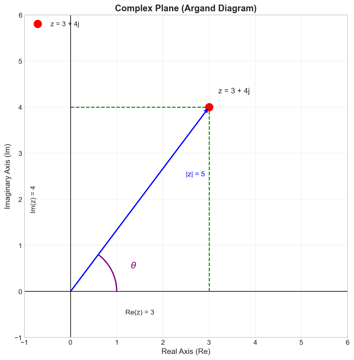
The Complex Plane

Complex numbers are visualized on the complex plane (Argand diagram), where the horizontal axis represents the real part and the vertical axis represents the imaginary part.

Properties

Equality: Two complex numbers are equal if and only if their real and imaginary parts are equal:

$$z_1=z_2⟺\text{Re}(z_1)=\text{Re}(z_2)\text{ and }\text{Im}(z_1)=\text{Im}(z_2)$$

Complex Conjugate: The complex conjugate of $z=x+jy$ is:

$$z^{\ast }=\overline{z}=x-jy$$

Python Implementation

import numpy as np

# Define a complex number
z = 3 + 4j

# Extract real and imaginary parts
print(f"z = {z}")
print(f"Real part: Re(z) = {z.real}")
print(f"Imaginary part: Im(z) = {z.imag}")
print(f"Complex conjugate: z* = {np.conj(z)}")

# Verify: z * z* = |z|²
print(f"z × z* = {z * np.conj(z)} = |z|² = {abs(z)**2}")

---

Polar Form

Definition

A complex number can also be expressed in polar form:

$$z=r(\cos \theta +j\sin \theta )$$

where:

• $r=|z|=\sqrt{x^2+y^2}$ is the magnitude (or modulus)
• $\theta =\mathrm{\angle }z=\arctan (y/x)$ is the phase (or argument)

Properties

Conversion from Rectangular:

$$r=\sqrt{x^2+y^2},\theta =\arctan \left(\frac{y}{x}\right)$$

(Note: Use atan2(y, x) in code to handle all quadrants correctly)

Conversion to Rectangular:

$$x=r\cos \theta ,y=r\sin \theta$$

Python Implementation

import numpy as np

z = 3 + 4j

# Magnitude and phase
r = np.abs(z)
theta = np.angle(z)  # in radians

print(f"z = {z}")
print(f"Magnitude: |z| = {r}")
print(f"Phase: θ = {theta:.4f} rad = {np.degrees(theta):.2f}°")

# Convert back to rectangular
x = r * np.cos(theta)
y = r * np.sin(theta)
z_reconstructed = x + 1j * y
print(f"Reconstructed: z = {z_reconstructed}")

---

Exponential Form and Euler's Formula

Euler's Formula

Euler's formula is one of the most important results in mathematics:

$$e^{j\theta }=\cos \theta +j\sin \theta$$

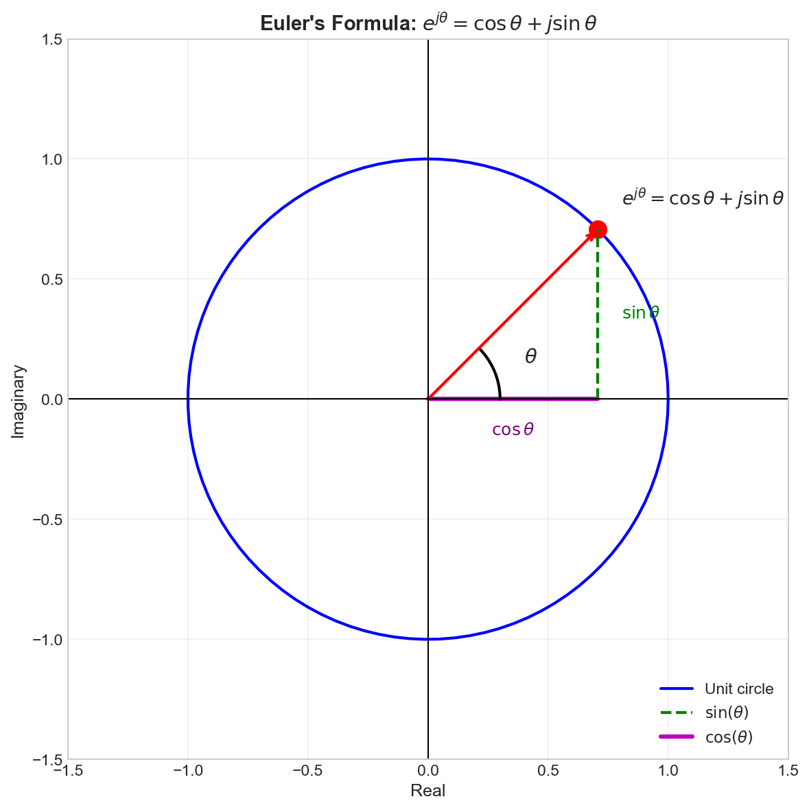
Properties

From Euler's formula, we can derive:

Cosine and Sine as Exponentials:

$$\cos \theta =\frac{e^{j\theta }+e^{-j\theta }}{2}$$$$\sin \theta =\frac{e^{j\theta }-e^{-j\theta }}{2j}$$

Exponential Form of Complex Numbers:

$$z=r{e}^{j\theta }$$

This combines magnitude and phase into a compact notation.

Python Implementation

import numpy as np
import matplotlib.pyplot as plt

# Verify Euler's formula
theta = np.pi / 4  # 45 degrees

euler_lhs = np.exp(1j * theta)
euler_rhs = np.cos(theta) + 1j * np.sin(theta)

print(f"e^(jθ) = {euler_lhs}")
print(f"cos(θ) + j·sin(θ) = {euler_rhs}")
print(f"Difference: {abs(euler_lhs - euler_rhs):.2e}")

# Express z = 3 + 4j in exponential form
z = 3 + 4j
r = np.abs(z)
theta = np.angle(z)
z_exp = r * np.exp(1j * theta)

print(f"\nz = {z}")
print(f"z = {r:.4f} × e^(j × {theta:.4f})")
print(f"Verification: {z_exp}")

---

Complex Arithmetic

Addition and Subtraction

Add/subtract real and imaginary parts separately:

$$(a+jb)+(c+jd)=(a+c)+j(b+d)$$$$(a+jb)-(c+jd)=(a-c)+j(b-d)$$

Multiplication

In rectangular form:

$$(a+jb)(c+jd)=(ac-bd)+j(ad+bc)$$

In polar/exponential form (more elegant):

$$r_1{e}^{j{\theta }_1}\cdot r_2{e}^{j{\theta }_2}=r_1{r}_2{e}^{j({\theta }_1+{\theta }_2)}$$

Magnitudes multiply, phases add.

Division

In rectangular form:

$$\frac{a+jb}{c+jd}=\frac{(a+jb)(c-jd)}{(c+jd)(c-jd)}=\frac{(ac+bd)+j(bc-ad)}{c^2+d^2}$$

In polar/exponential form:

$$\frac{r_1{e}^{j{\theta }_1}}{r_2{e}^{j{\theta }_2}}=\frac{r_1}{r_2}{e}^{j({\theta }_1-{\theta }_2)}$$

Magnitudes divide, phases subtract.

Python Implementation

import numpy as np

z1 = 3 + 4j
z2 = 1 + 2j

# Basic operations
print(f"z1 = {z1}")
print(f"z2 = {z2}")
print(f"z1 + z2 = {z1 + z2}")
print(f"z1 - z2 = {z1 - z2}")
print(f"z1 × z2 = {z1 * z2}")
print(f"z1 / z2 = {z1 / z2}")

# Verify multiplication rule: |z1 × z2| = |z1| × |z2|
print(f"\n|z1 × z2| = {np.abs(z1 * z2):.4f}")
print(f"|z1| × |z2| = {np.abs(z1) * np.abs(z2):.4f}")

# Verify: angle(z1 × z2) = angle(z1) + angle(z2)
print(f"\nangle(z1 × z2) = {np.angle(z1 * z2):.4f}")
print(f"angle(z1) + angle(z2) = {np.angle(z1) + np.angle(z2):.4f}")

---

Complex Exponentials and Rotation

The Unit Circle

The complex exponential $e^{j\theta }$ traces the unit circle as $\theta$ varies:

$$|e^{j\theta }|=1\text{for all }\theta$$

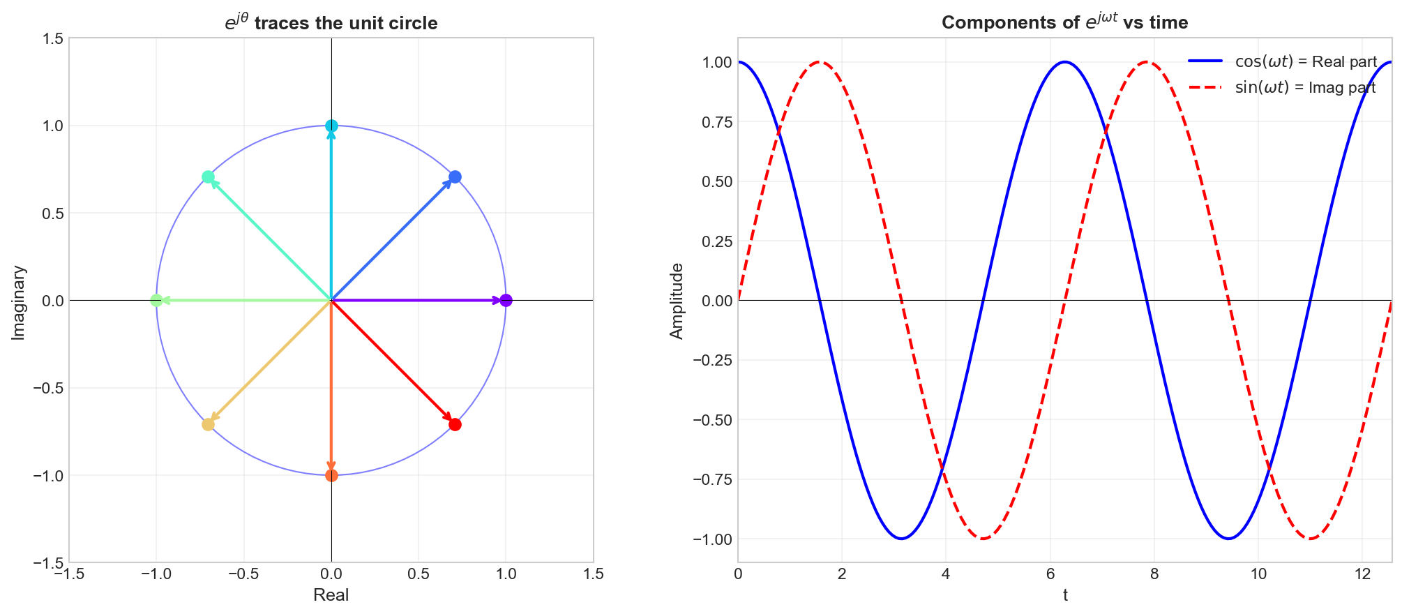
Properties

Rotating Phasor: $e^{j\omega t}$ represents a point rotating counterclockwise on the unit circle with angular velocity $\omega$.

Periodicity:

$$e^{j(\theta +2\pi )}=e^{j\theta }$$

De Moivre's Theorem:

$$(e^{j\theta }{)}^n=e^{jn\theta }=\cos (n\theta )+j\sin (n\theta )$$

Python Implementation

import numpy as np
import matplotlib.pyplot as plt

# e^(jωt) traces the unit circle
t = np.linspace(0, 2*np.pi, 100)
omega = 1
z = np.exp(1j * omega * t)

plt.figure(figsize=(10, 5))

# Left: trajectory in complex plane
plt.subplot(1, 2, 1)
plt.plot(np.real(z), np.imag(z), 'b-', linewidth=2)
plt.plot(1, 0, 'ro', markersize=10, label='Start (t=0)')
plt.xlabel('Real')
plt.ylabel('Imaginary')
plt.title(r'$e^{j\omega t}$ on Complex Plane')
plt.axis('equal')
plt.grid(True)
plt.legend()

# Right: real and imaginary parts vs time
plt.subplot(1, 2, 2)
plt.plot(t, np.real(z), 'b-', linewidth=2, label=r'$\cos(\omega t)$')
plt.plot(t, np.imag(z), 'r--', linewidth=2, label=r'$\sin(\omega t)$')
plt.xlabel('t')
plt.ylabel('Amplitude')
plt.title(r'Components of $e^{j\omega t}$')
plt.legend()
plt.grid(True)

plt.tight_layout()
plt.show()

Key Formulas

Formula	Expression
Euler's formula	$e^{j\theta }=\cos \theta +j\sin \theta$
Magnitude	$|z|=\sqrt{x^2+y^2}=\sqrt{z\cdot z^{\ast }}$
Phase	$\mathrm{\angle }z=\arctan (y/x)$
Conjugate	$(x+jy{)}^{\ast }=x-jy$
Cosine	$\cos \theta =\frac{e^{j\theta }+e^{-j\theta }}{2}$
Sine	$\sin \theta =\frac{e^{j\theta }-e^{-j\theta }}{2j}$