Calculus Essentials

Calculus is the mathematical language for describing change and accumulation. In signal processing, differentiation describes how signals change over time, while integration computes energy, averages, and transforms.

Differentiation

Definition

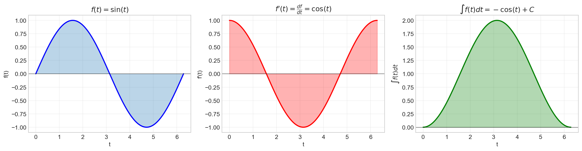
The derivative of a function $f(t)$ is defined as:

$$\frac{df}{dt}=f^{\prime }(t)=\underset{\mathrm{\Delta }t\to 0}{lim}\frac{f(t+\mathrm{\Delta }t)-f(t)}{\mathrm{\Delta }t}$$

The derivative represents the instantaneous rate of change of $f$ with respect to $t$.

Properties

Linearity:

$$\frac{d}{dt}[af(t)+bg(t)]=a\frac{df}{dt}+b\frac{dg}{dt}$$

Product Rule:

$$\frac{d}{dt}[f(t)g(t)]=f^{\prime }(t)g(t)+f(t)g^{\prime }(t)$$

Chain Rule:

$$\frac{d}{dt}[f(g(t))]=f^{\prime }(g(t))\cdot g^{\prime }(t)$$

Common Derivatives

Function $f(t)$	Derivative $f^{\prime }(t)$
$c$ (constant)	$0$
$t^n$	$n{t}^{n-1}$
$e^{at}$	$a{e}^{at}$
$\sin (\omega t)$	$\omega \cos (\omega t)$
$\cos (\omega t)$	$-\omega \sin (\omega t)$
$e^{j\omega t}$	$j\omega e^{j\omega t}$
$\ln (t)$	$1/t$

Python Implementation

import numpy as np
import matplotlib.pyplot as plt

# Numerical differentiation
def numerical_derivative(f, t, dt=1e-6):
    """Compute derivative using central difference."""
    return (f(t + dt) - f(t - dt)) / (2 * dt)

# Example: f(t) = sin(2πt)
t = np.linspace(0, 2, 200)
omega = 2 * np.pi

f = np.sin(omega * t)
df_analytical = omega * np.cos(omega * t)
df_numerical = numerical_derivative(lambda x: np.sin(omega * x), t)

plt.figure(figsize=(10, 4))
plt.plot(t, f, 'b-', linewidth=2, label=r'$f(t) = \sin(2\pi t)$')
plt.plot(t, df_analytical, 'r-', linewidth=2, label=r"$f'(t) = 2\pi\cos(2\pi t)$")
plt.plot(t, df_numerical, 'g--', linewidth=2, label='Numerical derivative')
plt.xlabel('t')
plt.ylabel('Amplitude')
plt.title('Function and Its Derivative')
plt.legend()
plt.grid(True)
plt.show()

---

Integration

Definition

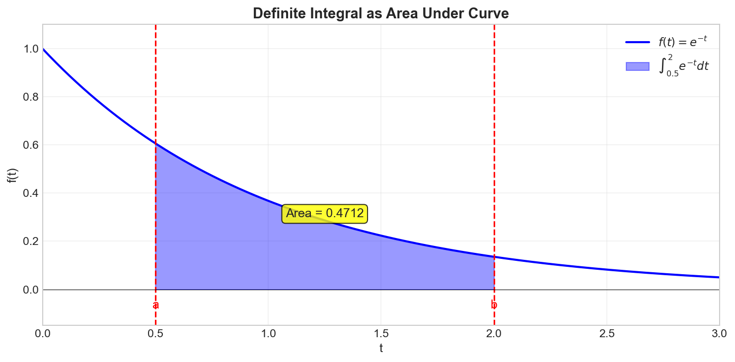
The definite integral of $f(t)$ from $a$ to $b$ is:

$${\int }_a^{b}f(t)dt=F(b)-F(a)$$

where $F(t)$ is the antiderivative (primitive) of $f(t)$, i.e., $F^{\prime }(t)=f(t)$.

The integral represents the signed area under the curve.

Properties

Linearity:

$$\int [af(t)+bg(t)]dt=a\int f(t)dt+b\int g(t)dt$$

Additivity over intervals:

$${\int }_a^{c}f(t)dt={\int }_a^{b}f(t)dt+{\int }_b^{c}f(t)dt$$

Integration by parts:

$$\int udv=uv-\int vdu$$

Common Integrals

Function $f(t)$	Integral $\int f(t)dt$
$t^n$ ($n\ne -1$)	$\frac{t^{n+1}}{n+1}$
$1/t$	$\ln |t|$
$e^{at}$	$\frac{1}{a}{e}^{at}$
$\sin (\omega t)$	$-\frac{1}{\omega }\cos (\omega t)$
$\cos (\omega t)$	$\frac{1}{\omega }\sin (\omega t)$
$e^{j\omega t}$	$\frac{1}{j\omega }{e}^{j\omega t}$

Python Implementation

import numpy as np
from scipy import integrate

# Numerical integration
def f(t):
    return np.exp(-t)

# Definite integral from 0 to infinity
result, error = integrate.quad(f, 0, np.inf)
print(f"∫₀^∞ e^(-t) dt = {result:.6f} (analytical: 1)")

# Numerical integration using trapezoidal rule
t = np.linspace(0, 10, 1000)
dt = t[1] - t[0]
y = f(t)
integral_trapz = np.trapz(y, t)
print(f"Trapezoidal approximation: {integral_trapz:.6f}")

# Cumulative integral (running integral)
cumulative = integrate.cumulative_trapezoid(y, t, initial=0)

import matplotlib.pyplot as plt
plt.figure(figsize=(10, 4))
plt.subplot(1, 2, 1)
plt.plot(t, y, 'b-', linewidth=2)
plt.fill_between(t, y, alpha=0.3)
plt.xlabel('t')
plt.ylabel('f(t)')
plt.title(r'$f(t) = e^{-t}$')
plt.grid(True)

plt.subplot(1, 2, 2)
plt.plot(t, cumulative, 'r-', linewidth=2)
plt.xlabel('t')
plt.ylabel(r'$\int_0^t f(\tau) d\tau$')
plt.title('Cumulative Integral')
plt.grid(True)
plt.axhline(y=1, color='k', linestyle='--', label='Limit = 1')
plt.legend()

plt.tight_layout()
plt.show()

---

Important Integrals in Signal Processing

Gaussian Integral

$${\int }_{-\mathrm{\infty }}^{+\mathrm{\infty }}{e}^{-a{x}^2}dx=\sqrt{\frac{\pi }{a}},a>0$$

Sinc Integral

$${\int }_{-\mathrm{\infty }}^{+\mathrm{\infty }}\text{sinc}(t)dt={\int }_{-\mathrm{\infty }}^{+\mathrm{\infty }}\frac{\sin (\pi t)}{\pi t}dt=1$$

Exponential Integral

$${\int }_0^{\mathrm{\infty }}{e}^{-at}dt=\frac{1}{a},a>0$$$${\int }_0^{\mathrm{\infty }}{t}^n{e}^{-at}dt=\frac{n!}{a^{n+1}},a>0$$

Python Implementation

import numpy as np
from scipy import integrate

# Gaussian integral: ∫ exp(-ax²) dx = √(π/a)
a = 2.0
result, _ = integrate.quad(lambda x: np.exp(-a * x**2), -np.inf, np.inf)
analytical = np.sqrt(np.pi / a)
print(f"Gaussian integral (a={a}): {result:.6f}, analytical: {analytical:.6f}")

# Sinc integral: ∫ sinc(t) dt = 1
result, _ = integrate.quad(np.sinc, -100, 100)
print(f"Sinc integral: {result:.6f} (analytical: 1)")

# Exponential moments: ∫₀^∞ t^n e^(-at) dt = n!/a^(n+1)
a = 1.0
for n in range(4):
    result, _ = integrate.quad(lambda t: t**n * np.exp(-a * t), 0, np.inf)
    analytical = np.math.factorial(n) / a**(n+1)
    print(f"n={n}: ∫ t^{n} e^(-t) dt = {result:.4f} (analytical: {analytical:.4f})")

---

Improper Integrals and Convergence

Definition

An improper integral has infinite limits or an unbounded integrand:

$${\int }_{-\mathrm{\infty }}^{+\mathrm{\infty }}f(t)dt=\underset{a\to -\mathrm{\infty }}{lim}\underset{b\to +\mathrm{\infty }}{lim}{\int }_a^{b}f(t)dt$$

Properties

Absolute Convergence: If $\int |f(t)|dt<\mathrm{\infty }$, then $\int f(t)dt$ converges absolutely.

Energy Signals: A signal has finite energy if:

$$E={\int }_{-\mathrm{\infty }}^{+\mathrm{\infty }}|x(t){|}^{2}dt<\mathrm{\infty }$$

Python Implementation

import numpy as np
from scipy import integrate

def signal_energy(x_func, t_min=-100, t_max=100):
    """Compute energy of a signal."""
    integrand = lambda t: np.abs(x_func(t))**2
    energy, _ = integrate.quad(integrand, t_min, t_max)
    return energy

# Decaying exponential (energy signal)
x1 = lambda t: np.exp(-np.abs(t))
E1 = signal_energy(x1)
print(f"Energy of e^(-|t|): {E1:.4f} (analytical: 1)")

# Gaussian (energy signal)
x2 = lambda t: np.exp(-np.pi * t**2)
E2 = signal_energy(x2)
print(f"Energy of exp(-πt²): {E2:.4f} (analytical: 1/√2 ≈ {1/np.sqrt(2):.4f})")

---

Taylor and Maclaurin Series

Definition

The Taylor series of $f(t)$ about $t=a$ is:

$$f(t)=\sum _{n=0}^{\mathrm{\infty }}\frac{f^{(n)}(a)}{n!}(t-a{)}^n$$

When $a=0$, this is the Maclaurin series.

Properties

Important series expansions:

Exponential:

$$e^t=\sum _{n=0}^{\mathrm{\infty }}\frac{t^n}{n!}=1+t+\frac{t^2}{2!}+\frac{t^3}{3!}+\cdots$$

Sine:

$$\sin (t)=\sum _{n=0}^{\mathrm{\infty }}\frac{(-1{)}^n{t}^{2n+1}}{(2n+1)!}=t-\frac{t^3}{3!}+\frac{t^5}{5!}-\cdots$$

Cosine:

$$\cos (t)=\sum _{n=0}^{\mathrm{\infty }}\frac{(-1{)}^n{t}^{2n}}{(2n)!}=1-\frac{t^2}{2!}+\frac{t^4}{4!}-\cdots$$

These series prove Euler's formula:

$$e^{jt}=\sum _{n=0}^{\mathrm{\infty }}\frac{(jt{)}^n}{n!}=\cos (t)+j\sin (t)$$

Python Implementation

import numpy as np
import matplotlib.pyplot as plt
from math import factorial

def taylor_exp(t, n_terms):
    """Taylor series approximation of e^t."""
    return sum(t**n / factorial(n) for n in range(n_terms))

def taylor_sin(t, n_terms):
    """Taylor series approximation of sin(t)."""
    return sum((-1)**n * t**(2*n+1) / factorial(2*n+1) for n in range(n_terms))

t = np.linspace(-3, 3, 200)

plt.figure(figsize=(12, 4))

# Exponential approximation
plt.subplot(1, 2, 1)
plt.plot(t, np.exp(t), 'k-', linewidth=2, label='exp(t)')
for n in [1, 2, 3, 5]:
    y = np.array([taylor_exp(ti, n) for ti in t])
    plt.plot(t, y, '--', label=f'{n} terms')
plt.ylim([-1, 10])
plt.xlabel('t')
plt.ylabel('f(t)')
plt.title('Taylor Series of exp(t)')
plt.legend()
plt.grid(True)

# Sine approximation
plt.subplot(1, 2, 2)
plt.plot(t, np.sin(t), 'k-', linewidth=2, label='sin(t)')
for n in [1, 2, 3, 5]:
    y = np.array([taylor_sin(ti, n) for ti in t])
    plt.plot(t, y, '--', label=f'{n} terms')
plt.ylim([-2, 2])
plt.xlabel('t')
plt.ylabel('f(t)')
plt.title('Taylor Series of sin(t)')
plt.legend()
plt.grid(True)

plt.tight_layout()
plt.show()

---

Summary

Differentiation Rules

Rule	Formula
Constant	$(cf{)}^{\prime }=c{f}^{\prime }$
Sum	$(f+g{)}^{\prime }=f^{\prime }+g^{\prime }$
Product	$(fg{)}^{\prime }=f^{\prime }g+f{g}^{\prime }$
Quotient	$(f/g{)}^{\prime }=(f^{\prime }g-f{g}^{\prime })/g^2$
Chain	$(f(g){)}^{\prime }=f^{\prime }(g)\cdot g^{\prime }$

Key Integrals for Signal Processing

Integral	Value
${\int }_{-\mathrm{\infty }}^{\mathrm{\infty }}{e}^{-a{x}^2}dx$	$\sqrt{\pi /a}$
${\int }_0^{\mathrm{\infty }}{e}^{-at}dt$	$1/a$
${\int }_0^{\mathrm{\infty }}t{e}^{-at}dt$	$1/a^2$
${\int }_{-\mathrm{\infty }}^{\mathrm{\infty }}\text{sinc}(t)dt$	$1$
${\int }_0^T{\sin }^2(\omega t)dt$	$T/2$ (if $\omega T=2\pi n$)