Linear Algebra

Linear algebra provides the mathematical framework for representing signals as vectors, understanding transformations, and analyzing multi-dimensional systems. These concepts are essential for understanding the Fourier transform, filter design, and state-space analysis.

Vectors

Definition

A vector $\mathbf{v}$ in ${\mathbb{R}}^n$ (or ${\mathbb{C}}^n$ for complex vectors) is an ordered collection of $n$ numbers:

$$\mathbf{v}=\left[\begin{array}{c}{v}_1\\ v_2\\ ⋮\\ v_n\end{array}\right]$$

In signal processing, a discrete signal $x[n]$ for $n=0,1,\dots ,N-1$ can be represented as a vector:

$$\mathbf{x}=\left[\begin{array}{c}x[0]\\ x[1]\\ ⋮\\ x[N-1]\end{array}\right]$$

Properties

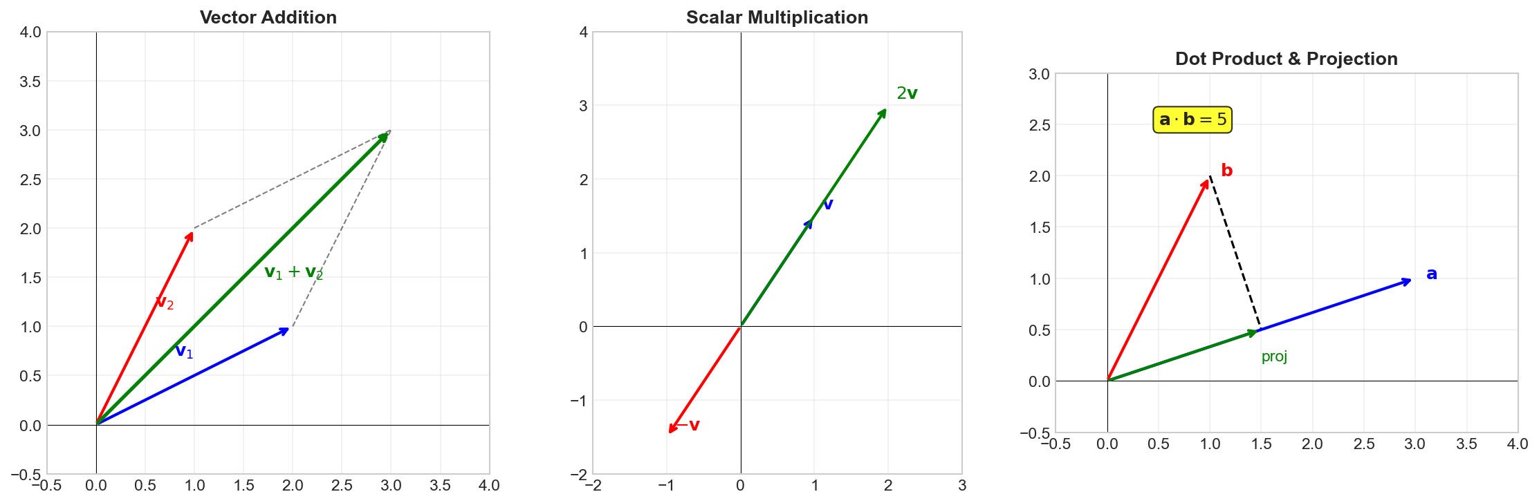
Vector Addition:

$$\mathbf{u}+\mathbf{v}=\left[\begin{array}{c}{u}_1+v_1\\ u_2+v_2\\ ⋮\\ u_n+v_n\end{array}\right]$$

Scalar Multiplication:

$$c\mathbf{v}=\left[\begin{array}{c}c{v}_1\\ c{v}_2\\ ⋮\\ c{v}_n\end{array}\right]$$

Linear Combination: A vector $\mathbf{w}$ is a linear combination of vectors ${\mathbf{v}}_1,\dots ,{\mathbf{v}}_k$ if:

$$\mathbf{w}=c_1{\mathbf{v}}_1+c_2{\mathbf{v}}_2+\cdots +c_k{\mathbf{v}}_k$$

Linear Independence: Vectors ${\mathbf{v}}_1,\dots ,{\mathbf{v}}_k$ are linearly independent if the only solution to:

$$c_1{\mathbf{v}}_1+c_2{\mathbf{v}}_2+\cdots +c_k{\mathbf{v}}_k=\mathbf{0}$$

is $c_1=c_2=\cdots =c_k=0$.

Python Implementation

import numpy as np

# Define vectors
v1 = np.array([1, 2, 3])
v2 = np.array([4, 5, 6])

# Vector operations
print(f"v1 = {v1}")
print(f"v2 = {v2}")
print(f"v1 + v2 = {v1 + v2}")
print(f"2 * v1 = {2 * v1}")

# Linear combination
c1, c2 = 0.5, 0.3
w = c1 * v1 + c2 * v2
print(f"\n{c1}*v1 + {c2}*v2 = {w}")

# Check linear independence using rank
V = np.column_stack([v1, v2])
rank = np.linalg.matrix_rank(V)
print(f"\nMatrix rank: {rank}")
print(f"Vectors are {'linearly independent' if rank == 2 else 'linearly dependent'}")

---

Inner Products and Norms

Definition

The inner product (dot product) of two real vectors $\mathbf{u},\mathbf{v}\in {\mathbb{R}}^n$ is:

$$⟨\mathbf{u},\mathbf{v}⟩={\mathbf{u}}^T\mathbf{v}=\sum _{i=1}^n{u}_i{v}_i$$

For complex vectors $\mathbf{u},\mathbf{v}\in {\mathbb{C}}^n$:

$$⟨\mathbf{u},\mathbf{v}⟩={\mathbf{u}}^H\mathbf{v}=\sum _{i=1}^n{u}_i^{\ast }{v}_i$$

where ${\mathbf{u}}^H=({\mathbf{u}}^{\ast }{)}^T$ is the conjugate transpose (Hermitian transpose).

The norm (length) of a vector is:

$$\parallel \mathbf{v}\parallel =\sqrt{⟨\mathbf{v},\mathbf{v}⟩}=\sqrt{\sum _{i=1}^n|v_i{|}^2}$$

Properties

Cauchy-Schwarz Inequality:

$$|⟨\mathbf{u},\mathbf{v}⟩|\le \parallel \mathbf{u}\parallel \cdot \parallel \mathbf{v}\parallel$$

Orthogonality: Two vectors are orthogonal if $⟨\mathbf{u},\mathbf{v}⟩=0$.

Angle Between Vectors:

$$\cos \theta =\frac{⟨\mathbf{u},\mathbf{v}⟩}{\parallel \mathbf{u}\parallel \cdot \parallel \mathbf{v}\parallel }$$

Parseval's Theorem: For an orthonormal basis $\{{\mathbf{e}}_1,\dots ,{\mathbf{e}}_n\}$:

$$\parallel \mathbf{v}{\parallel }^2=\sum _{i=1}^n|⟨\mathbf{v},{\mathbf{e}}_i⟩{|}^2$$

Python Implementation

import numpy as np

# Real vectors
u = np.array([1, 2, 3])
v = np.array([4, 5, 6])

# Inner product and norm
inner_product = np.dot(u, v)
norm_u = np.linalg.norm(u)
norm_v = np.linalg.norm(v)

print(f"u = {u}")
print(f"v = {v}")
print(f"<u, v> = {inner_product}")
print(f"||u|| = {norm_u:.4f}")
print(f"||v|| = {norm_v:.4f}")

# Angle between vectors
cos_theta = inner_product / (norm_u * norm_v)
theta = np.arccos(cos_theta)
print(f"\nAngle between u and v: {np.degrees(theta):.2f}°")

# Complex vectors
u_complex = np.array([1 + 1j, 2 - 1j])
v_complex = np.array([1 - 1j, 1 + 1j])

# Hermitian inner product: u^H * v
inner_complex = np.vdot(u_complex, v_complex)
print(f"\nComplex inner product: {inner_complex}")

# Orthogonal vectors example
e1 = np.array([1, 0, 0])
e2 = np.array([0, 1, 0])
print(f"\n<e1, e2> = {np.dot(e1, e2)} (orthogonal)")

---

Matrices

Definition

A matrix $\mathbf{A}$ is a rectangular array of numbers with $m$ rows and $n$ columns:

$$\mathbf{A}=\left[\begin{array}{cccc}{a}_{11}& a_{12}& \cdots & a_{1n}\\ a_{21}& a_{22}& \cdots & a_{2n}\\ ⋮& ⋮& \ddots & ⋮\\ a_{m1}& a_{m2}& \cdots & a_{mn}\end{array}\right]\in {\mathbb{R}}^{m\times n}$$

Properties

Matrix-Vector Multiplication: For $\mathbf{A}\in {\mathbb{R}}^{m\times n}$ and $\mathbf{x}\in {\mathbb{R}}^n$:

$$\mathbf{y}=\mathbf{A}\mathbf{x},y_i=\sum _{j=1}^n{a}_{ij}{x}_j$$

Matrix-Matrix Multiplication: For $\mathbf{A}\in {\mathbb{R}}^{m\times n}$ and $\mathbf{B}\in {\mathbb{R}}^{n\times p}$:

$$\mathbf{C}=\mathbf{A}\mathbf{B},c_{ij}=\sum _{k=1}^n{a}_{ik}{b}_{kj}$$

Transpose: $({\mathbf{A}}^T{)}_{ij}=a_{ji}$

Important Identities:

• $(\mathbf{A}\mathbf{B}{)}^T={\mathbf{B}}^T{\mathbf{A}}^T$
• $({\mathbf{A}}^{-1}{)}^T=({\mathbf{A}}^T{)}^{-1}$

Python Implementation

import numpy as np

# Define a matrix
A = np.array([[1, 2, 3],
              [4, 5, 6]])

# Matrix properties
print(f"A =\n{A}")
print(f"Shape: {A.shape}")
print(f"Transpose:\n{A.T}")

# Matrix-vector multiplication
x = np.array([1, 0, -1])
y = A @ x  # or np.dot(A, x)
print(f"\nx = {x}")
print(f"A @ x = {y}")

# Matrix-matrix multiplication
B = np.array([[1, 2],
              [3, 4],
              [5, 6]])
C = A @ B
print(f"\nB =\n{B}")
print(f"A @ B =\n{C}")

# Verify (AB)^T = B^T A^T
print(f"\n(AB)^T =\n{C.T}")
print(f"B^T A^T =\n{B.T @ A.T}")

---

Special Matrices

Definition

Several special matrix types appear frequently in signal processing:

Identity Matrix:

$$\mathbf{I}=\left[\begin{array}{cccc}1& 0& \cdots & 0\\ 0& 1& \cdots & 0\\ ⋮& ⋮& \ddots & ⋮\\ 0& 0& \cdots & 1\end{array}\right]$$

Diagonal Matrix:

$$\mathbf{D}=\text{diag}(d_1,d_2,\dots ,d_n)=\left[\begin{array}{cccc}{d}_1& 0& \cdots & 0\\ 0& d_2& \cdots & 0\\ ⋮& ⋮& \ddots & ⋮\\ 0& 0& \cdots & d_n\end{array}\right]$$

Symmetric Matrix: ${\mathbf{A}}^T=\mathbf{A}$

Hermitian Matrix: ${\mathbf{A}}^H=\mathbf{A}$ (for complex matrices)

Orthogonal Matrix: ${\mathbf{Q}}^T\mathbf{Q}=\mathbf{Q}{\mathbf{Q}}^T=\mathbf{I}$

Unitary Matrix: ${\mathbf{U}}^H\mathbf{U}=\mathbf{U}{\mathbf{U}}^H=\mathbf{I}$ (for complex matrices)

Properties

Orthogonal/Unitary matrices preserve norms:

$$\parallel \mathbf{Q}\mathbf{x}\parallel =\parallel \mathbf{x}\parallel$$

Toeplitz Matrix: Constant diagonals (appears in convolution):

$$\mathbf{T}=\left[\begin{array}{ccc}{t}_0& t_{-1}& t_{-2}\\ t_1& t_0& t_{-1}\\ t_2& t_1& t_0\end{array}\right]$$

Circulant Matrix: Toeplitz with circular structure (appears in DFT):

$$\mathbf{C}=\left[\begin{array}{cccc}{c}_0& c_{N-1}& \cdots & c_1\\ c_1& c_0& \cdots & c_2\\ ⋮& ⋮& \ddots & ⋮\\ c_{N-1}& c_{N-2}& \cdots & c_0\end{array}\right]$$

Python Implementation

import numpy as np
from scipy.linalg import toeplitz, circulant

# Identity matrix
I = np.eye(3)
print(f"Identity matrix:\n{I}")

# Diagonal matrix
D = np.diag([1, 2, 3])
print(f"\nDiagonal matrix:\n{D}")

# Symmetric matrix
A = np.array([[1, 2, 3],
              [2, 4, 5],
              [3, 5, 6]])
print(f"\nSymmetric matrix:\n{A}")
print(f"A == A^T: {np.allclose(A, A.T)}")

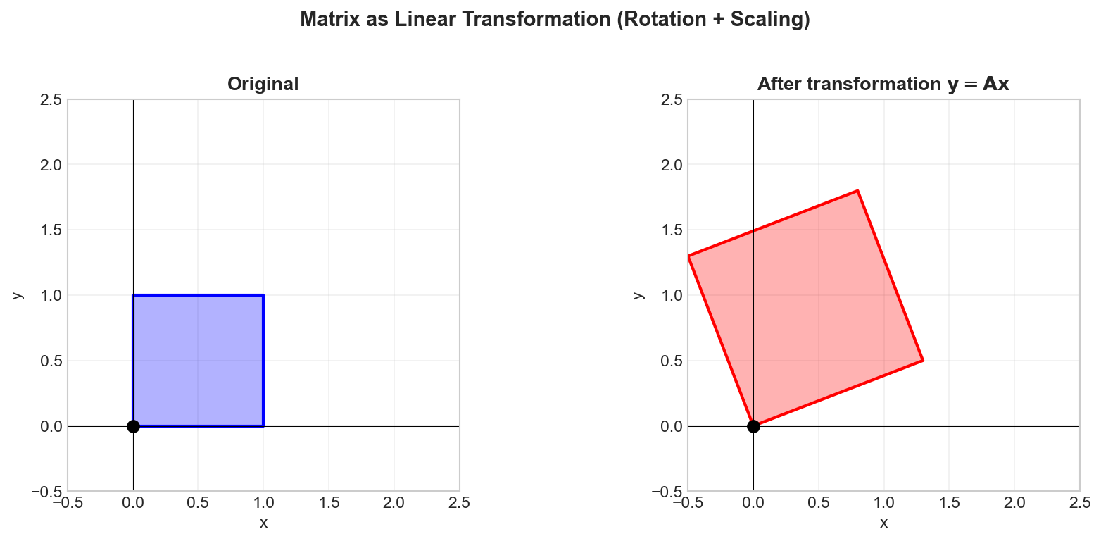
# Orthogonal matrix (rotation)
theta = np.pi / 4
Q = np.array([[np.cos(theta), -np.sin(theta)],
              [np.sin(theta), np.cos(theta)]])
print(f"\nOrthogonal matrix (rotation by 45°):\n{Q}")
print(f"Q^T @ Q =\n{Q.T @ Q}")

# Verify norm preservation
x = np.array([1, 2])
print(f"\n||x|| = {np.linalg.norm(x):.4f}")
print(f"||Qx|| = {np.linalg.norm(Q @ x):.4f}")

# Toeplitz matrix (convolution structure)
c = [1, 2, 3]  # first column
r = [1, 4, 5]  # first row
T = toeplitz(c, r)
print(f"\nToeplitz matrix:\n{T}")

# Circulant matrix (DFT structure)
c = [1, 2, 3, 4]
C = circulant(c)
print(f"\nCirculant matrix:\n{C}")

---

Eigenvalues and Eigenvectors

Definition

For a square matrix $\mathbf{A}\in {\mathbb{R}}^{n\times n}$, a scalar $\lambda$ is an eigenvalue and a non-zero vector $\mathbf{v}$ is the corresponding eigenvector if:

$$\mathbf{A}\mathbf{v}=\lambda \mathbf{v}$$

Eigenvalues are found by solving the characteristic equation:

$$det(\mathbf{A}-\lambda \mathbf{I})=0$$

Properties

Eigendecomposition: If $\mathbf{A}$ has $n$ linearly independent eigenvectors:

$$\mathbf{A}=\mathbf{V}\mathbf{\Lambda }{\mathbf{V}}^{-1}$$

where $\mathbf{V}$ contains eigenvectors as columns and $\mathbf{\Lambda }=\text{diag}({\lambda }_1,\dots ,{\lambda }_n)$.

Spectral Properties:

• $\text{trace}(\mathbf{A})=\sum _i{\lambda }_i$
• $det(\mathbf{A})=\prod _i{\lambda }_i$
• Eigenvalues of ${\mathbf{A}}^k$ are ${\lambda }_i^k$

Symmetric Matrices:

• All eigenvalues are real
• Eigenvectors are orthogonal
• $\mathbf{A}=\mathbf{Q}\mathbf{\Lambda }{\mathbf{Q}}^T$ where $\mathbf{Q}$ is orthogonal

Python Implementation

import numpy as np
import matplotlib.pyplot as plt

# Define a matrix
A = np.array([[4, 2],
              [1, 3]])

# Compute eigenvalues and eigenvectors
eigenvalues, eigenvectors = np.linalg.eig(A)

print(f"A =\n{A}")
print(f"\nEigenvalues: {eigenvalues}")
print(f"\nEigenvectors (columns):\n{eigenvectors}")

# Verify: A @ v = lambda * v
for i in range(len(eigenvalues)):
    v = eigenvectors[:, i]
    lam = eigenvalues[i]
    Av = A @ v
    lam_v = lam * v
    print(f"\nEigenpair {i+1}:")
    print(f"  A @ v = {Av}")
    print(f"  λ * v = {lam_v}")
    print(f"  Match: {np.allclose(Av, lam_v)}")

# Eigendecomposition
V = eigenvectors
Lambda = np.diag(eigenvalues)
A_reconstructed = V @ Lambda @ np.linalg.inv(V)
print(f"\nV @ Λ @ V⁻¹ =\n{A_reconstructed.real}")

# Symmetric matrix example
S = np.array([[3, 1],
              [1, 3]])
eig_vals, eig_vecs = np.linalg.eigh(S)  # use eigh for symmetric matrices
print(f"\nSymmetric matrix S =\n{S}")
print(f"Eigenvalues: {eig_vals}")
print(f"Eigenvectors are orthogonal: {np.allclose(eig_vecs.T @ eig_vecs, np.eye(2))}")

---

Matrix Inverse and Determinant

Definition

The inverse of a square matrix $\mathbf{A}$ is a matrix ${\mathbf{A}}^{-1}$ such that:

$$\mathbf{A}{\mathbf{A}}^{-1}={\mathbf{A}}^{-1}\mathbf{A}=\mathbf{I}$$

A matrix is invertible (non-singular) if and only if $det(\mathbf{A})\ne 0$.

The determinant for a $2\times 2$ matrix:

$$det\left[\begin{array}{cc}a& b\\ c& d\end{array}\right]=ad-bc$$

Properties

Inverse of Products:

$$(\mathbf{A}\mathbf{B}{)}^{-1}={\mathbf{B}}^{-1}{\mathbf{A}}^{-1}$$

Determinant of Products:

$$det(\mathbf{A}\mathbf{B})=det(\mathbf{A})det(\mathbf{B})$$

Linear Systems: To solve $\mathbf{A}\mathbf{x}=\mathbf{b}$:

$$\mathbf{x}={\mathbf{A}}^{-1}\mathbf{b}$$

(In practice, use LU decomposition or other numerical methods)

Python Implementation

import numpy as np

# Define a matrix
A = np.array([[4, 7],
              [2, 6]])

# Determinant
det_A = np.linalg.det(A)
print(f"A =\n{A}")
print(f"det(A) = {det_A:.4f}")

# Inverse
A_inv = np.linalg.inv(A)
print(f"\nA⁻¹ =\n{A_inv}")

# Verify: A @ A^(-1) = I
print(f"\nA @ A⁻¹ =\n{A @ A_inv}")

# Solve linear system Ax = b
b = np.array([1, 2])
x = np.linalg.solve(A, b)  # more numerically stable than inv(A) @ b
print(f"\nSolving Ax = b where b = {b}")
print(f"x = {x}")
print(f"Verification: A @ x = {A @ x}")

# Singular matrix (det = 0)
B = np.array([[1, 2],
              [2, 4]])
det_B = np.linalg.det(B)
print(f"\nSingular matrix B =\n{B}")
print(f"det(B) = {det_B:.6f}")

---

Orthogonality and Projections

Definition

A set of vectors $\{{\mathbf{v}}_1,\dots ,{\mathbf{v}}_k\}$ is orthonormal if:

$$⟨{\mathbf{v}}_i,{\mathbf{v}}_j⟩={\delta }_{ij}=\{\begin{array}{ll}1& \text{if }i=j\\ 0& \text{if }i\ne j\end{array}$$

The orthogonal projection of $\mathbf{v}$ onto $\mathbf{u}$ is:

$${\text{proj}}_{\mathbf{u}}(\mathbf{v})=\frac{⟨\mathbf{v},\mathbf{u}⟩}{⟨\mathbf{u},\mathbf{u}⟩}\mathbf{u}$$

Properties

Gram-Schmidt Process: Converts a set of linearly independent vectors into an orthonormal set.

Orthogonal Complement: For a subspace $W$, its orthogonal complement $W^{\perp }$ contains all vectors orthogonal to every vector in $W$.

Projection Matrix: The projection onto the column space of $\mathbf{A}$ is:

$$\mathbf{P}=\mathbf{A}({\mathbf{A}}^T\mathbf{A}{)}^{-1}{\mathbf{A}}^T$$

Python Implementation

import numpy as np

def gram_schmidt(V):
    """Gram-Schmidt orthonormalization."""
    n = V.shape[1]
    Q = np.zeros_like(V, dtype=float)

    for i in range(n):
        q = V[:, i].astype(float)
        for j in range(i):
            q = q - np.dot(Q[:, j], V[:, i]) * Q[:, j]
        Q[:, i] = q / np.linalg.norm(q)

    return Q

# Example vectors
v1 = np.array([1, 1, 0])
v2 = np.array([1, 0, 1])
v3 = np.array([0, 1, 1])
V = np.column_stack([v1, v2, v3])

print(f"Original vectors (columns):\n{V}")

# Orthonormalize
Q = gram_schmidt(V)
print(f"\nOrthonormalized vectors:\n{Q}")

# Verify orthonormality
print(f"\nQ^T @ Q (should be identity):\n{np.round(Q.T @ Q, 10)}")

# Projection onto a vector
u = np.array([1, 0, 0])
v = np.array([3, 4, 0])
proj = (np.dot(v, u) / np.dot(u, u)) * u
print(f"\nProjection of v={v} onto u={u}: {proj}")

# Projection matrix onto column space of A
A = np.array([[1, 0],
              [0, 1],
              [1, 1]])
P = A @ np.linalg.inv(A.T @ A) @ A.T
print(f"\nProjection matrix P:\n{P}")

# Project a vector
y = np.array([1, 2, 3])
y_proj = P @ y
print(f"\nProjection of y={y} onto col(A): {y_proj}")

---

The DFT Matrix

Definition

The Discrete Fourier Transform can be expressed as a matrix-vector multiplication. The DFT matrix ${\mathbf{F}}_N$ is:

$${\mathbf{F}}_N=\left[\begin{array}{ccccc}1& 1& 1& \cdots & 1\\ 1& W_N& W_N^2& \cdots & W_N^{N-1}\\ 1& W_N^2& W_N^4& \cdots & W_N^{2(N-1)}\\ ⋮& ⋮& ⋮& \ddots & ⋮\\ 1& W_N^{N-1}& W_N^{2(N-1)}& \cdots & W_N^{(N-1{)}^2}\end{array}\right]$$

where $W_N=e^{-j2\pi /N}$ is the primitive $N$-th root of unity.

The DFT of a signal $\mathbf{x}$ is:

$$\mathbf{X}={\mathbf{F}}_N\mathbf{x}$$

Properties

Unitary Property: The normalized DFT matrix $\frac{1}{\sqrt{N}}{\mathbf{F}}_N$ is unitary:

$${\mathbf{F}}_N^H{\mathbf{F}}_N=N\mathbf{I}$$

Inverse DFT:

$$\mathbf{x}=\frac{1}{N}{\mathbf{F}}_N^H\mathbf{X}$$

Circulant Matrix Diagonalization: The DFT diagonalizes circulant matrices:

$$\mathbf{C}={\mathbf{F}}_N^{-1}\mathbf{\Lambda }{\mathbf{F}}_N$$

Python Implementation

import numpy as np

def dft_matrix(N):
    """Construct the N-point DFT matrix."""
    n = np.arange(N)
    k = n.reshape((N, 1))
    W = np.exp(-2j * np.pi * k * n / N)
    return W

# Create 4-point DFT matrix
N = 4
F = dft_matrix(N)
print(f"DFT matrix F_{N}:\n{np.round(F, 4)}")

# Verify: F^H @ F = N * I
print(f"\nF^H @ F / N (should be identity):\n{np.round(F.conj().T @ F / N, 10).real}")

# Compare with numpy FFT
x = np.array([1, 2, 3, 4])
X_matrix = F @ x
X_fft = np.fft.fft(x)

print(f"\nSignal x = {x}")
print(f"DFT via matrix: {np.round(X_matrix, 4)}")
print(f"DFT via FFT:    {np.round(X_fft, 4)}")

# Inverse DFT
x_recovered = F.conj().T @ X_matrix / N
print(f"\nRecovered signal: {np.round(x_recovered.real, 4)}")

# Diagonalization of circulant matrix
from scipy.linalg import circulant
c = [1, 2, 0, 0]
C = circulant(c)
print(f"\nCirculant matrix C:\n{C}")

# Eigenvalues are DFT of first column
eigenvalues_theory = np.fft.fft(c)
eigenvalues_actual = np.linalg.eigvals(C)
print(f"\nEigenvalues from DFT: {np.round(eigenvalues_theory, 4)}")
print(f"Actual eigenvalues:   {np.round(np.sort(eigenvalues_actual), 4)}")

---

Summary

Vector Operations

Operation	Formula
Inner product	$⟨\mathbf{u},\mathbf{v}⟩={\mathbf{u}}^T\mathbf{v}$
Norm	$|\mathbf{v}|=\sqrt{⟨\mathbf{v},\mathbf{v}⟩}$
Projection	${\text{proj}}_{\mathbf{u}}(\mathbf{v})=\frac{⟨\mathbf{v},\mathbf{u}⟩}{|\mathbf{u}{|}^2}\mathbf{u}$

Matrix Properties

Property	Condition
Symmetric	${\mathbf{A}}^T=\mathbf{A}$
Orthogonal	${\mathbf{Q}}^T\mathbf{Q}=\mathbf{I}$
Unitary	${\mathbf{U}}^H\mathbf{U}=\mathbf{I}$
Invertible	$det(\mathbf{A})\ne 0$

Key Decompositions

Decomposition	Form	Application
Eigendecomposition	$\mathbf{A}=\mathbf{V}\mathbf{\Lambda }{\mathbf{V}}^{-1}$	System analysis
Spectral (symmetric)	$\mathbf{A}=\mathbf{Q}\mathbf{\Lambda }{\mathbf{Q}}^T$	Signal energy
DFT	$\mathbf{X}={\mathbf{F}}_N\mathbf{x}$	Frequency analysis