Chapter 2: LTI Systems

This chapter introduces Linear Time-Invariant (LTI) systems, which form the cornerstone of signal processing theory. Their mathematical tractability and widespread applicability make them essential for understanding signal analysis and system design.

This chapter focuses on LTI SISO systems (Single-Input Single-Output). The theory extends to MIMO systems through state-space representations and matrix transfer functions, which are covered in advanced courses.

Linearity

Definition

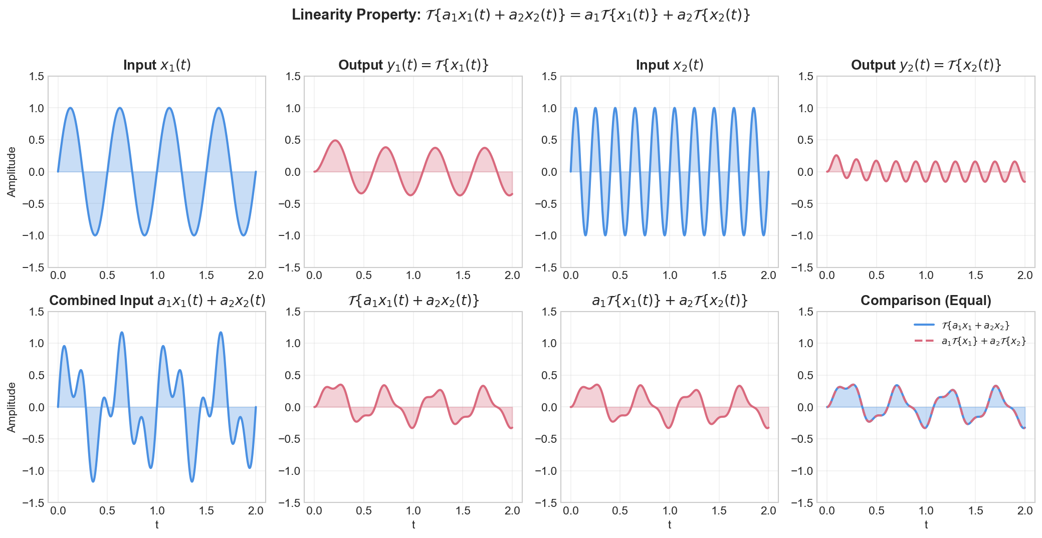
A system is linear if it satisfies the superposition principle:

$$\mathcal{T}\{a_1{x}_1(t)+a_2{x}_2(t)\}=a_1\mathcal{T}\{x_1(t)\}+a_2\mathcal{T}\{x_2(t)\}$$

for all signals $x_1(t)$, $x_2(t)$ and constants $a_1$, $a_2$.

This property combines two conditions:

• Additivity: $\mathcal{T}\{x_1(t)+x_2(t)\}=\mathcal{T}\{x_1(t)\}+\mathcal{T}\{x_2(t)\}$
• Homogeneity (Scaling): $\mathcal{T}\{ax(t)\}=a\mathcal{T}\{x(t)\}$

Illustration

Time-Invariance

Definition

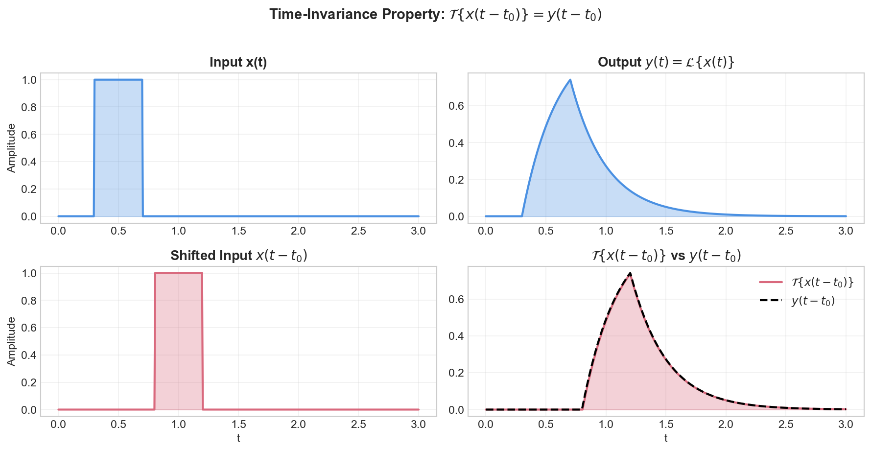
A system is time-invariant if a time shift in the input causes an identical time shift in the output:

$$\text{If }y(t)=\mathcal{T}\{x(t)\},\text{ then }y(t-t_0)=\mathcal{T}\{x(t-t_0)\}$$

In other words, the system's behavior does not change over time.

Illustration

Impulse Response

Definition

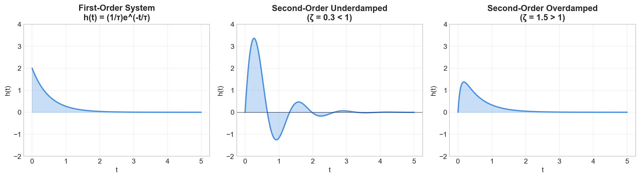
The impulse response $h(t)$ of an LTI system is the output when the input is a Dirac delta function:

$$h(t)=\mathcal{T}\{\delta (t)\}$$

The impulse response completely characterizes an LTI system.

Properties

Causality: A system is causal if and only if:

$$h(t)=0\text{for }t<0$$

BIBO Stability: A system is Bounded-Input Bounded-Output stable if and only if:

$${\int }_{-\mathrm{\infty }}^{+\mathrm{\infty }}|h(t)|dt<\mathrm{\infty }$$

Convolution

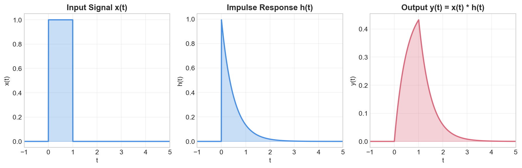
Definition

An LTI system is completely characterized by its impulse response. Given any input $x(t)$, the output is obtained through convolution:

$$y(t)=x(t)\ast h(t)={\int }_{-\mathrm{\infty }}^{+\mathrm{\infty }}x(\tau )h(t-\tau )d\tau$$

Demonstration

Add proof

Properties

Commutativity:

$$x(t)\ast h(t)=h(t)\ast x(t)$$

Associativity:

$$[x(t)\ast h_1(t)]\ast h_2(t)=x(t)\ast [h_1(t)\ast h_2(t)]$$

Distributivity:

$$x(t)\ast [h_1(t)+h_2(t)]=x(t)\ast h_1(t)+x(t)\ast h_2(t)$$

Identity:

$$x(t)\ast \delta (t)=x(t)$$

Shift:

$$x(t)\ast \delta (t-t_0)=x(t-t_0)$$

Frequency Response

Definition

The frequency response $H(j\omega )$ describes how an LTI system responds to sinusoidal inputs at different frequencies. It is the Fourier transform of the impulse response:

$$H(j\omega )={\int }_{-\mathrm{\infty }}^{+\mathrm{\infty }}h(t)e^{-j\omega t}dt$$

The frequency response can be written in polar form:

$$H(j\omega )=|H(j\omega )|e^{j\mathrm{\angle }H(j\omega )}$$

where:

• $|H(j\omega )|$ is the magnitude response (gain)
• $\mathrm{\angle }H(j\omega )$ is the phase response

Properties

Eigenfunction Property: Complex exponentials are eigenfunctions of LTI systems:

$$\mathcal{T}\{e^{j\omega t}\}=H(j\omega )e^{j\omega t}$$

Sinusoidal Steady-State Response: For input $x(t)=A\cos ({\omega }_{0}t+\varphi )$:

$$y(t)=A|H(j{\omega }_0)|\cos ({\omega }_{0}t+\varphi +\mathrm{\angle }H(j{\omega }_0))$$

The output is a sinusoid at the same frequency, with amplitude scaled by $|H(j{\omega }_0)|$ and phase shifted by $\mathrm{\angle }H(j{\omega }_0)$.

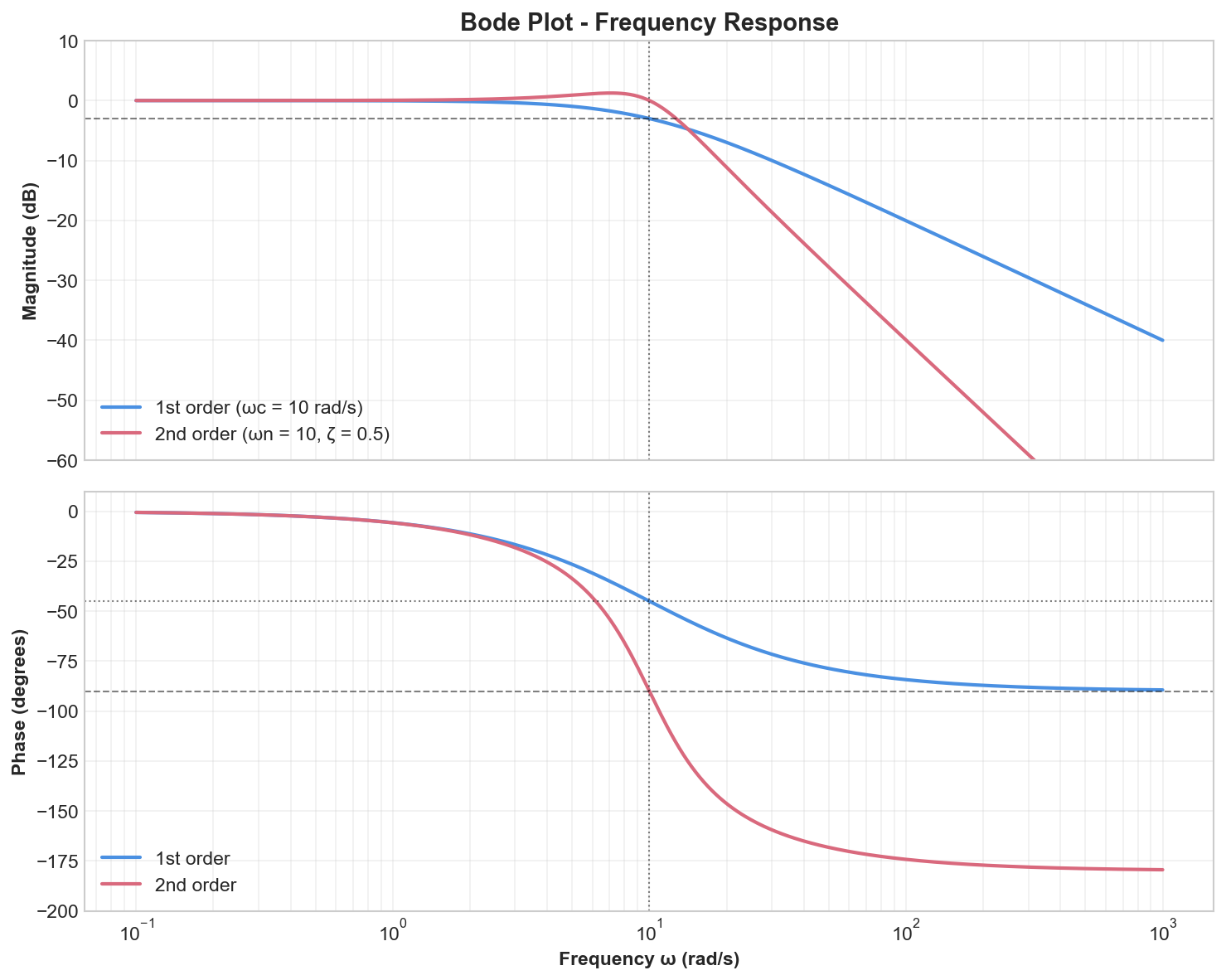
Bode Plot

The Bode plot displays the magnitude (in dB) and phase of the frequency response versus frequency on a logarithmic scale:

• Magnitude: $20{\log }_{10}|H(j\omega )|$ in dB
• Phase: $\mathrm{\angle }H(j\omega )$ in degrees

Causality and Stability

Causality

A system is causal if the output at any time depends only on present and past inputs (not future inputs).

For LTI systems: A system is causal if and only if:

$$h(t)=0\text{for }t<0$$

BIBO Stability

A system is Bounded-Input Bounded-Output (BIBO) stable if every bounded input produces a bounded output.

For LTI systems: A system is BIBO stable if and only if the impulse response is absolutely integrable:

$${\int }_{-\mathrm{\infty }}^{+\mathrm{\infty }}|h(t)|dt<\mathrm{\infty }$$

Summary

Property	Definition	LTI System Criterion
Linearity	$\mathcal{T}\{a{x}_1+b{x}_2\}=a\mathcal{T}\{x_1\}+b\mathcal{T}\{x_2\}$	Superposition holds
Time-Invariance	$\mathcal{T}\{x(t-t_0)\}=y(t-t_0)$	Shift in → Shift out
Causality	Output depends only on past/present	$h(t)=0$ for $t<0$
BIBO Stability	Bounded input → Bounded output	$\int |h(t)|dt<\mathrm{\infty }$

Key Results:

1. LTI systems are completely characterized by their impulse response $h(t)$
2. Output is computed via convolution: $y(t)=x(t)\ast h(t)$
3. Frequency response $H(j\omega )=\mathcal{F}\{h(t)\}$ describes sinusoidal steady-state behavior
4. Convolution in time ↔ Multiplication in frequency