Chapter 4: Fourier Transform

Introduction

The Fourier series is a powerful tool for analyzing periodic signals, but many real-world signals are aperiodic (non-periodic). To analyze these signals, we extend the Fourier series to create the Fourier Transform. This chapter introduces the Fourier Transform and demonstrates how it emerges naturally from the Fourier series as the period approaches infinity.

From Fourier Series to Fourier Transform

The Fourier series is limited to periodic signals. To analyze aperiodic (non-periodic) signals, we extend the Fourier series by letting the period $T_0\to \mathrm{\infty }$.

Intuition: As the period increases, an aperiodic signal can be viewed as a periodic signal with infinite period. The fundamental frequency ${\omega }_0=2\pi /T_0$ becomes infinitesimal, and the discrete line spectrum becomes a continuous spectrum.

Derivation:

Starting from the Fourier series:

$$x(t)=\sum _{k=-\mathrm{\infty }}^{+\mathrm{\infty }}{c}_k{e}^{jk{\omega }_{0}t}$$

where

$$c_k=\frac{1}{T_0}{\int }_{-T_0/2}^{T_0/2}x(t)e^{-jk{\omega }_{0}t}dt$$

Substituting $c_k$ into the series:

$$x(t)=\sum _{k=-\mathrm{\infty }}^{+\mathrm{\infty }}[\frac{1}{T_0}{\int }_{-T_0/2}^{T_0/2}x(\tau )e^{-jk{\omega }_0\tau }d\tau ]e^{jk{\omega }_{0}t}$$$$=\frac{1}{2\pi }\sum _{k=-\mathrm{\infty }}^{+\mathrm{\infty }}[{\int }_{-T_0/2}^{T_0/2}x(\tau )e^{-jk{\omega }_0\tau }d\tau ]e^{jk{\omega }_{0}t}{\omega }_0$$

As $T_0\to \mathrm{\infty }$:

• ${\omega }_0=2\pi /T_0\to d\omega$ (becomes infinitesimal)
• $k{\omega }_0\to \omega$ (discrete frequencies become continuous)
• $\sum _{k=-\mathrm{\infty }}^{+\mathrm{\infty }}(\cdot ){\omega }_0\to {\int }_{-\mathrm{\infty }}^{+\mathrm{\infty }}(\cdot )d\omega$ (sum becomes integral)
• Integration limits: $\pm T_0/2\to \pm \mathrm{\infty }$

This yields:

$$x(t)=\frac{1}{2\pi }{\int }_{-\mathrm{\infty }}^{+\mathrm{\infty }}[{\int }_{-\mathrm{\infty }}^{+\mathrm{\infty }}x(\tau )e^{-j\omega \tau }d\tau ]e^{j\omega t}d\omega$$

Fourier Transform Pair

Definition: Fourier Transform and Inverse Fourier Transform

For an aperiodic signal $x(t)$, the Fourier Transform is:

$$X(\omega )=\mathcal{F}\{x(t)\}={\int }_{-\mathrm{\infty }}^{+\mathrm{\infty }}x(t)e^{-j\omega t}dt$$

and the Inverse Fourier Transform is:

$$x(t)={\mathcal{F}}^{-1}\{X(\omega )\}=\frac{1}{2\pi }{\int }_{-\mathrm{\infty }}^{+\mathrm{\infty }}X(\omega )e^{j\omega t}d\omega$$

We write: $x(t)\stackrel{\mathcal{F}}{\leftrightarrow }X(\omega )$

Notation:

• $X(\omega )$ is called the spectrum or frequency spectrum of $x(t)$
• $\omega$ is the angular frequency in rad/s
• Alternatively, using $f$ in Hz: $X(f)={\int }_{-\mathrm{\infty }}^{+\mathrm{\infty }}x(t)e^{-j2\pi ft}dt$

Properties of the Fourier Transform

Proposition: Basic Properties

For real signals $x(t)$:

• Conjugate symmetry: $X(-\omega )=X^{\ast }(\omega )$
• Even magnitude: $|X(-\omega )|=|X(\omega )|$
• Odd phase: $\mathrm{\angle }X(-\omega )=-\mathrm{\angle }X(\omega )$

Proposition: Linearity

$$a{x}_1(t)+b{x}_2(t)\stackrel{\mathcal{F}}{\leftrightarrow }a{X}_1(\omega )+b{X}_2(\omega )$$

Proposition: Time Shift

$$x(t-t_0)\stackrel{\mathcal{F}}{\leftrightarrow }{e}^{-j\omega t_0}X(\omega )$$

Proposition: Frequency Shift (Modulation)

$$x(t)e^{j{\omega }_{0}t}\stackrel{\mathcal{F}}{\leftrightarrow }X(\omega -{\omega }_0)$$

Proposition: Time Scaling

$$x(at)\stackrel{\mathcal{F}}{\leftrightarrow }\frac{1}{|a|}X\left(\frac{\omega }{a}\right)$$

Proposition: Differentiation in Time

$$\frac{dx(t)}{dt}\stackrel{\mathcal{F}}{\leftrightarrow }j\omega X(\omega )$$

Proposition: Convolution

$$x(t)\ast y(t)\stackrel{\mathcal{F}}{\leftrightarrow }X(\omega )Y(\omega )$$

Proposition: Parseval's Theorem

$${\int }_{-\mathrm{\infty }}^{+\mathrm{\infty }}|x(t){|}^{2}dt=\frac{1}{2\pi }{\int }_{-\mathrm{\infty }}^{+\mathrm{\infty }}|X(\omega ){|}^{2}d\omega$$

Representation: Continuous Spectrum

Unlike the Fourier series which produces a discrete line spectrum, the Fourier Transform produces a continuous spectrum.

Definition: Magnitude and Phase Spectrum

For a signal $x(t)$ with Fourier Transform $X(\omega )$:

1. Magnitude Spectrum: $|X(\omega )|$ - shows the amplitude of each frequency component
2. Phase Spectrum: $\mathrm{\angle }X(\omega )$ - shows the phase shift of each frequency component

Key Differences from Fourier Series:

Aspect	Fourier Series	Fourier Transform
Signal Type	Periodic	Aperiodic
Spectrum	Discrete (line spectrum)	Continuous
Frequency Variable	$k{\omega }_0$ (discrete)	$\omega$ (continuous)
Coefficients	$c_k$ (dimensionless)	$X(\omega )$ (has units)
Representation	Sum over harmonics	Integral over frequencies

Interpretation:

• $X(\omega )$ represents the density of frequency components at frequency $\omega$
• The magnitude $|X(\omega )|$ shows how much of frequency $\omega$ is present in the signal
• The phase $\mathrm{\angle }X(\omega )$ shows the phase relationship of each frequency component
• Energy is distributed continuously across the frequency spectrum
• Wider signals in time → narrower spectra in frequency (time-bandwidth relationship)

Visualization Example:

The continuous spectrum is typically visualized as a continuous curve rather than discrete lines. For real signals, the magnitude spectrum is even and the phase spectrum is odd.

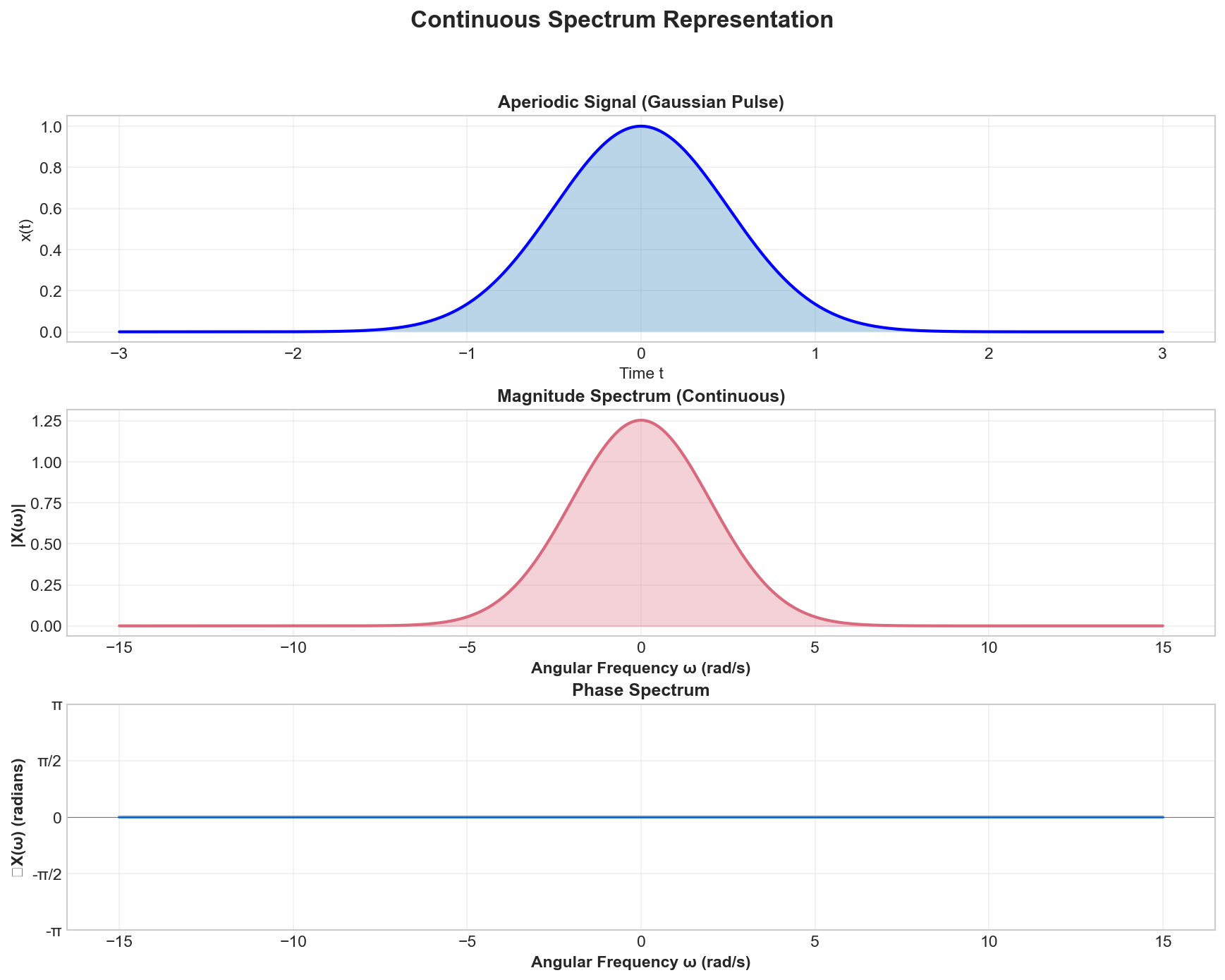
The figure illustrates a continuous spectrum for an aperiodic Gaussian pulse. Unlike the discrete line spectrum of periodic signals, the Fourier Transform produces a continuous frequency distribution. The magnitude spectrum (middle) shows the even symmetry property for real signals, and the phase spectrum (bottom) shows the odd symmetry. Notice that energy is distributed continuously across all frequencies, not just at discrete harmonics.

Fourier Transform of Periodic Signals

Link to Fourier Series

An interesting and important case occurs when we apply the Fourier Transform to a periodic signal. Although periodic signals have infinite energy and do not satisfy the standard conditions for the existence of the Fourier Transform, we can still define their Fourier Transform using the Dirac delta function (impulse function).

This establishes a direct connection between the Fourier Series (Chapter 3) and the Fourier Transform (Chapter 4).

Theorem: Fourier Transform of a Periodic Signal

Consider a periodic signal $x(t)$ with period $T_0$ and fundamental frequency ${\omega }_0=2\pi /T_0$. From Chapter 3, we know that $x(t)$ can be expressed as a complex exponential Fourier series:

$$x(t)=\sum _{k=-\mathrm{\infty }}^{+\mathrm{\infty }}{c}_k{e}^{jk{\omega }_{0}t}$$

where the Fourier series coefficients are:

$$c_k=\frac{1}{T_0}{\int }_{-T_0/2}^{T_0/2}x(t)e^{-jk{\omega }_{0}t}dt$$

The Fourier Transform of $x(t)$ is:

$$X(\omega )=2\pi \sum _{k=-\mathrm{\infty }}^{+\mathrm{\infty }}{c}_k\delta (\omega -k{\omega }_0)$$

Interpretation:

• The Fourier Transform of a periodic signal consists of impulses (Dirac delta functions) located at the harmonic frequencies $k{\omega }_0$
• The weight (area) of each impulse is $2\pi c_k$, where $c_k$ is the Fourier series coefficient from Chapter 3
• This converts the discrete line spectrum (Fourier Series) into a distribution of impulses (Fourier Transform)
• The line spectra from Chapter 3 (plot of $|c_k|$ vs $k$) corresponds directly to the impulse magnitudes in the Fourier Transform

Demonstration

Starting from the Fourier Series:

We know that:

$$x(t)=\sum _{k=-\mathrm{\infty }}^{+\mathrm{\infty }}{c}_k{e}^{jk{\omega }_{0}t}$$

Taking the Fourier Transform of both sides:

$$X(\omega )=\mathcal{F}\left\{\sum _{k=-\mathrm{\infty }}^{+\mathrm{\infty }}{c}_k{e}^{jk{\omega }_{0}t}\right\}$$

By linearity of the Fourier Transform:

$$X(\omega )=\sum _{k=-\mathrm{\infty }}^{+\mathrm{\infty }}{c}_k\mathcal{F}\left\{e^{jk{\omega }_{0}t}\right\}$$

Fourier Transform of a Complex Exponential:

We need to find $\mathcal{F}\{e^{j{\omega }_{0}t}\}$. Using the frequency shift property and the fact that $\mathcal{F}\{1\}=2\pi \delta (\omega )$:

$$\mathcal{F}\{e^{j{\omega }_{0}t}\}=2\pi \delta (\omega -{\omega }_0)$$

More generally:

$$\mathcal{F}\{e^{jk{\omega }_{0}t}\}=2\pi \delta (\omega -k{\omega }_0)$$

Final Result:

Substituting back:

$$X(\omega )=\sum _{k=-\mathrm{\infty }}^{+\mathrm{\infty }}{c}_k\cdot 2\pi \delta (\omega -k{\omega }_0)$$$$=2\pi \sum _{k=-\mathrm{\infty }}^{+\mathrm{\infty }}{c}_k\delta (\omega -k{\omega }_0)$$

This shows that the Fourier Transform of a periodic signal is a train of impulses at the harmonic frequencies, with weights proportional to the Fourier series coefficients.

Connection to Chapter 3:

Recall from Chapter 3 that the line spectrum represents:

• Magnitude spectrum: Plot of $|c_k|$ versus $k$ (or versus $k{\omega }_0$)
• Phase spectrum: Plot of $\mathrm{\angle }{c}_k$ versus $k$ (or versus $k{\omega }_0$)

The Fourier Transform representation gives us:

• Impulses at frequencies $\omega =k{\omega }_0$
• Impulse weights $2\pi c_k$ (or magnitude $2\pi |c_k|$ and phase $\mathrm{\angle }{c}_k$)

These are equivalent representations: the line spectrum shows discrete values at integer $k$, while the Fourier Transform shows impulses at the corresponding angular frequencies $k{\omega }_0$.

Example: Square Wave

Consider the square wave from Chapter 3, Example 1, with Fourier series:

$$x(t)=\sum _{k=-\mathrm{\infty }}^{+\mathrm{\infty }}{c}_k{e}^{jk{\omega }_{0}t}$$

where for odd $k$: $c_k=\frac{2A}{jk\pi }$ and for even $k\ne 0$: $c_k=0$, and $c_0=0$.

The Fourier Transform is:

$$X(\omega )=2\pi \sum _{\begin{array}{c}k\text{ odd}\end{array}}\frac{2A}{jk\pi }\delta (\omega -k{\omega }_0)=\sum _{\begin{array}{c}k\text{ odd}\end{array}}\frac{4A}{jk}\delta (\omega -k{\omega }_0)$$

This shows impulses at $\omega =\pm {\omega }_0,\pm 3{\omega }_0,\pm 5{\omega }_0,\dots$ with amplitudes decreasing as $1/k$.

Visualization:

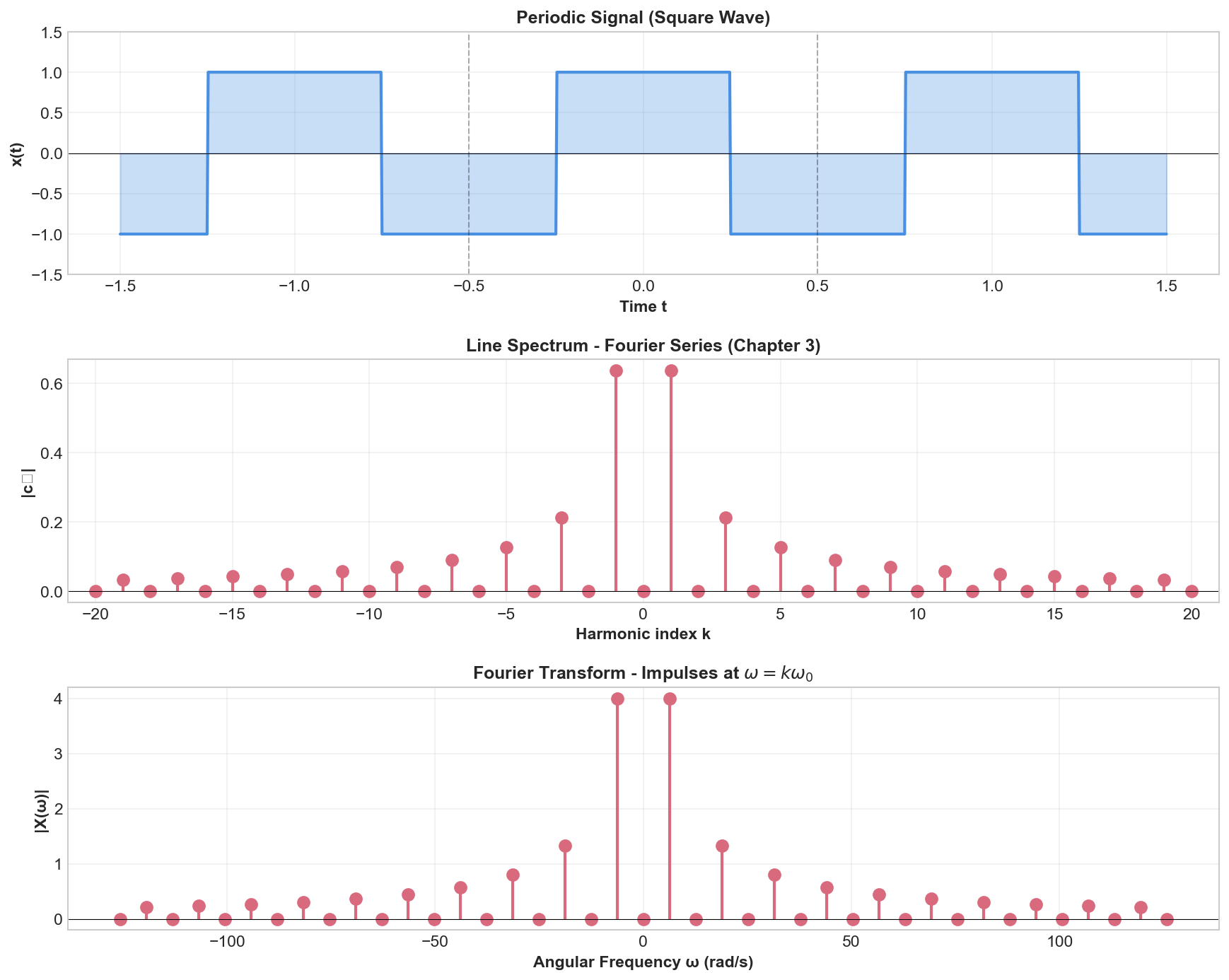
The figure compares the Fourier Series representation (line spectra from Chapter 3) with the Fourier Transform representation (impulses) for a periodic square wave. The top panel shows the periodic signal in time. The middle panel shows the discrete line spectrum from Chapter 3 (magnitude |c_k| versus k). The bottom panel shows the corresponding Fourier Transform with impulses at ω = kω₀, demonstrating that the two representations are equivalent: line spectra show discrete coefficients while the Fourier Transform shows impulses at the corresponding frequencies.

Key Points:

1. Periodic signals → Discrete spectrum (impulses at harmonics)
2. Aperiodic signals → Continuous spectrum
3. The Fourier Series coefficients $c_k$ from Chapter 3 directly determine the impulse weights in the Fourier Transform
4. As $T_0\to \mathrm{\infty }$ (signal becomes aperiodic), the impulses merge into a continuous spectrum
5. This connection shows that the Fourier Series is a special case of the Fourier Transform for periodic signals

Examples

Example 1: Rectangular Pulse (Porte)

Consider a rectangular pulse of width $\tau$ and amplitude $A$:

$$x(t)=\{\begin{array}{ll}A& |t|<\tau /2\\ 0& |t|>\tau /2\end{array}$$

This is also written as $x(t)=A\cdot \text{rect}(t/\tau )$ where $\text{rect}(t)$ is the rectangular function.

The Fourier transform is:

$$X(\omega )=A\tau \cdot \text{sinc}\left(\frac{\omega \tau }{2\pi }\right)=\frac{A\tau \sin (\omega \tau /2)}{\omega \tau /2}$$

or equivalently:

$$X(\omega )=A\tau \cdot \frac{\sin (\omega \tau /2)}{\omega \tau /2}$$

Demonstration

Compute the Fourier transform:

$$X(\omega )={\int }_{-\mathrm{\infty }}^{+\mathrm{\infty }}x(t)e^{-j\omega t}dt={\int }_{-\tau /2}^{\tau /2}A{e}^{-j\omega t}dt$$$$=A{\left[\frac{e^{-j\omega t}}{-j\omega }\right]}_{-\tau /2}^{\tau /2}=\frac{A}{-j\omega }(e^{-j\omega \tau /2}-e^{j\omega \tau /2})$$

Using Euler's formula: $e^{jx}-e^{-jx}=2j\sin (x)$

$$e^{j\omega \tau /2}-e^{-j\omega \tau /2}=2j\sin (\omega \tau /2)$$

Therefore:

$$X(\omega )=\frac{A}{-j\omega }\cdot (-2j\sin (\omega \tau /2))=\frac{2A\sin (\omega \tau /2)}{\omega }$$$$=A\tau \cdot \frac{\sin (\omega \tau /2)}{\omega \tau /2}$$

This can be written as:

$$X(\omega )=A\tau \cdot \text{sinc}\left(\frac{\omega \tau }{2\pi }\right)$$

where $\text{sinc}(x)=\frac{\sin (\pi x)}{\pi x}$ (normalized sinc function).

Key observations:

• $X(0)=A\tau$ (the DC value is the area under the pulse)
• The spectrum has zeros at $\omega =\pm 2\pi n/\tau$ for $n=1,2,3,\dots$
• The first zero crossing occurs at $\omega =2\pi /\tau$
• Narrower pulse (smaller $\tau$) → wider spectrum (inverse relationship)
• The spectrum decays as $1/\omega$ for large $\omega$

Visualization:

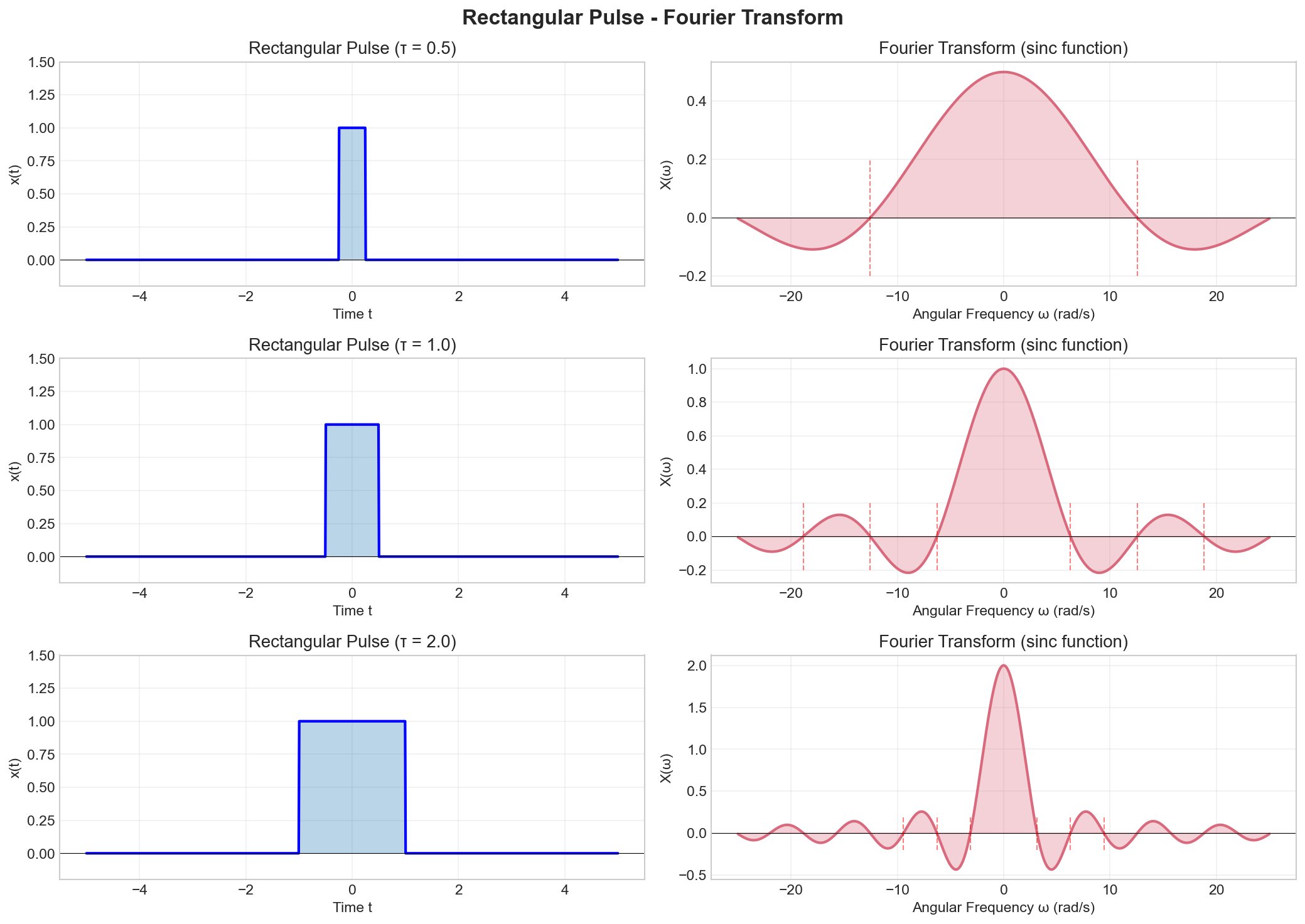
The figure shows rectangular pulses of different widths (τ = 0.5, 1.0, 2.0) and their corresponding Fourier transforms. The transform is a sinc function with zeros at ω = ±2πn/τ. Key observation: narrower pulses (smaller τ) have wider spectra, demonstrating the inverse time-frequency relationship. The first zero crossing moves further from the origin as the pulse becomes narrower.

Example 2: Exponential Decay (One-Sided)

Consider a one-sided exponential decay:

$$x(t)=\{\begin{array}{ll}{e}^{-at}& t\ge 0\\ 0& t<0\end{array},a>0$$

The Fourier transform is:

$$X(\omega )=\frac{1}{a+j\omega }$$

Demonstration

Compute the Fourier transform:

$$X(\omega )={\int }_{-\mathrm{\infty }}^{+\mathrm{\infty }}x(t)e^{-j\omega t}dt={\int }_0^{+\mathrm{\infty }}{e}^{-at}{e}^{-j\omega t}dt$$$$={\int }_0^{+\mathrm{\infty }}{e}^{-(a+j\omega )t}dt={\left[\frac{e^{-(a+j\omega )t}}{-(a+j\omega )}\right]}_0^{+\mathrm{\infty }}$$

For $a>0$, the exponential vanishes at infinity:

$$=\frac{1}{a+j\omega }(0-1)=\frac{1}{a+j\omega }$$

Magnitude and phase:

$$|X(\omega )|=\frac{1}{\sqrt{a^2+{\omega }^2}}$$$$\mathrm{\angle }X(\omega )=-\arctan \left(\frac{\omega }{a}\right)$$

Key observations:

• The magnitude spectrum is a Lorentzian (decreases as $1/\omega$ for large $\omega$)
• At $\omega =0$: $|X(0)|=1/a$
• At $\omega =a$: $|X(a)|=1/(\sqrt{2}a)$ (half-power point)
• Faster decay (larger $a$) → narrower spectrum

Visualization:

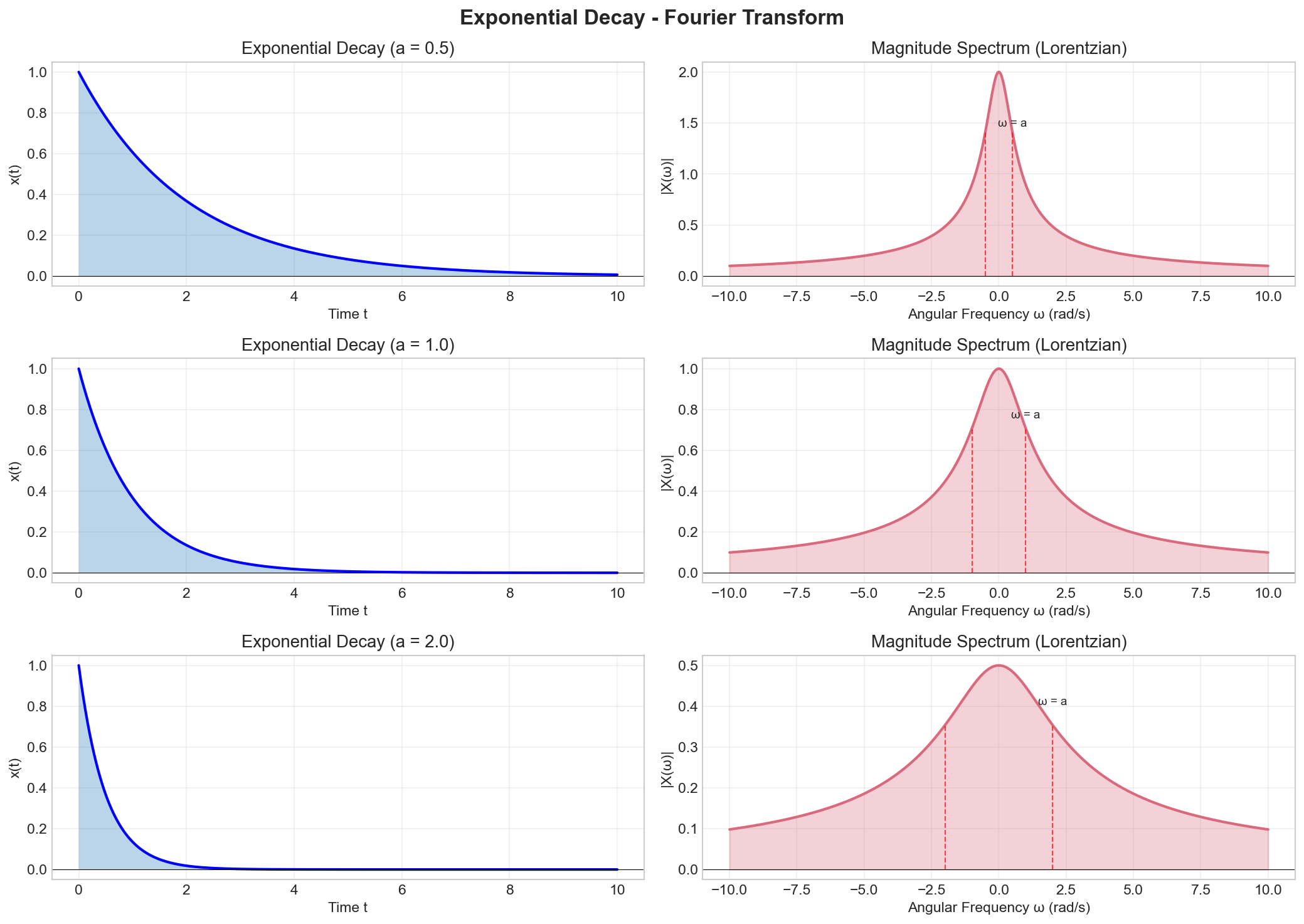
The figure shows exponential decays with different decay rates (a = 0.5, 1.0, 2.0) and their Lorentzian magnitude spectra. The half-power point occurs at ω = a, marked with dashed lines. Faster decay in time (larger a) leads to a wider spectrum in frequency, but the spectrum is still more concentrated at low frequencies. The Lorentzian shape is characteristic of exponential decay signals.

Example 3: Gaussian Pulse

Consider a Gaussian pulse:

$$x(t)=A{e}^{-t^2/(2{\sigma }^2)}$$

The Fourier transform is also Gaussian:

$$X(\omega )=A\sigma \sqrt{2\pi }{e}^{-{\sigma }^2{\omega }^2/2}$$

Demonstration

The Fourier transform of a Gaussian is well-known and can be computed using the property:

$${\int }_{-\mathrm{\infty }}^{+\mathrm{\infty }}{e}^{-a{x}^2+bx}dx=\sqrt{\frac{\pi }{a}}{e}^{b^2/(4a)}$$

Starting with:

$$X(\omega )={\int }_{-\mathrm{\infty }}^{+\mathrm{\infty }}A{e}^{-t^2/(2{\sigma }^2)}{e}^{-j\omega t}dt$$$$=A{\int }_{-\mathrm{\infty }}^{+\mathrm{\infty }}{e}^{-t^2/(2{\sigma }^2)-j\omega t}dt$$

Complete the square in the exponent:

$$-\frac{t^2}{2{\sigma }^2}-j\omega t=-\frac{1}{2{\sigma }^2}(t^2+2j{\sigma }^2\omega t)=-\frac{1}{2{\sigma }^2}[(t+j{\sigma }^2\omega {)}^2+{\sigma }^4{\omega }^2]$$$$=-\frac{(t+j{\sigma }^2\omega {)}^2}{2{\sigma }^2}-\frac{{\sigma }^2{\omega }^2}{2}$$

Therefore:

$$X(\omega )=A{e}^{-{\sigma }^2{\omega }^2/2}{\int }_{-\mathrm{\infty }}^{+\mathrm{\infty }}{e}^{-(t+j{\sigma }^2\omega {)}^2/(2{\sigma }^2)}dt$$

Using the substitution $u=t+j{\sigma }^2\omega$ and the Gaussian integral:

$${\int }_{-\mathrm{\infty }}^{+\mathrm{\infty }}{e}^{-u^2/(2{\sigma }^2)}du=\sigma \sqrt{2\pi }$$

We get:

$$X(\omega )=A\sigma \sqrt{2\pi }{e}^{-{\sigma }^2{\omega }^2/2}$$

Key observations:

• The Fourier transform of a Gaussian is also a Gaussian (self-reciprocal)
• Wider pulse (larger $\sigma$) → narrower spectrum (smaller $1/\sigma$ in frequency)
• This demonstrates the uncertainty principle: $\mathrm{\Delta }t\cdot \mathrm{\Delta }\omega \ge$ constant
• Gaussian has the minimum time-bandwidth product

Visualization:

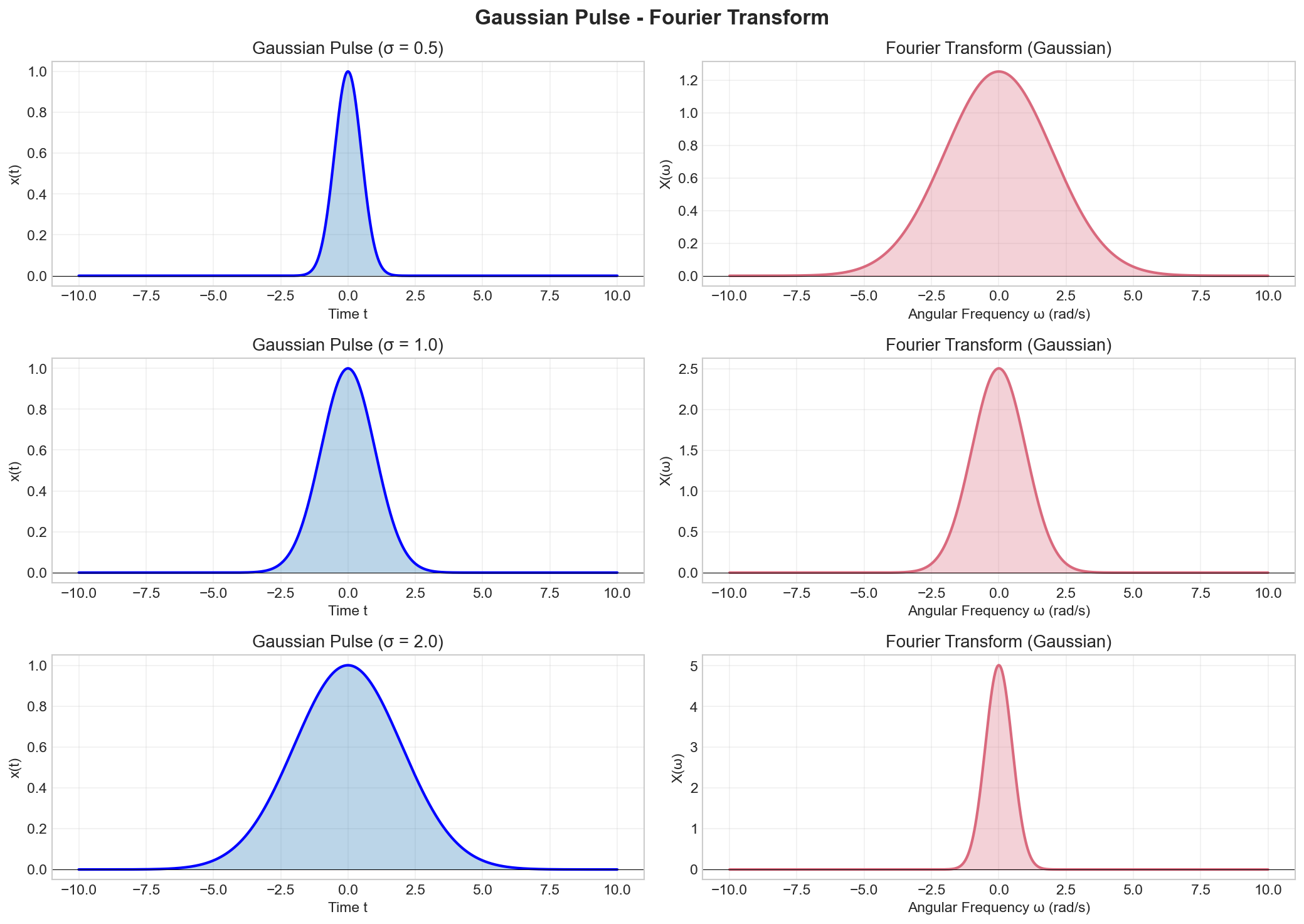
The figure shows Gaussian pulses with different widths (σ = 0.5, 1.0, 2.0) and their Gaussian Fourier transforms. This is a remarkable property: the Fourier transform of a Gaussian is also a Gaussian (self-reciprocal). The time-frequency duality is clearly visible: wider pulses in time (larger σ) produce narrower spectra in frequency. Gaussians achieve the minimum time-bandwidth product, making them optimal for localization in both domains simultaneously.

Example 4: Amplitude Modulated (AM) Signal

Consider an amplitude modulated signal where a carrier at frequency ${\omega }_c$ is modulated by a message signal:

$$x(t)=A(1+m\cos ({\omega }_{m}t))\cos ({\omega }_{c}t)$$

where:

• $A$ is the carrier amplitude
• $m$ is the modulation index (0 ≤ m ≤ 1)
• ${\omega }_m$ is the message frequency (low frequency)
• ${\omega }_c$ is the carrier frequency (high frequency, ${\omega }_c>>{\omega }_m$)

The Fourier transform is:

$$X(\omega )=A\pi [\delta (\omega -{\omega }_c)+\delta (\omega +{\omega }_c)]+\frac{Am\pi }{2}[\delta (\omega -{\omega }_c-{\omega }_m)+\delta (\omega -{\omega }_c+{\omega }_m)+\delta (\omega +{\omega }_c-{\omega }_m)+\delta (\omega +{\omega }_c+{\omega }_m)]$$

Demonstration

Expand the signal:

$$x(t)=A\cos ({\omega }_{c}t)+Am\cos ({\omega }_{m}t)\cos ({\omega }_{c}t)$$

Using the product-to-sum identity: $\cos (A)\cos (B)=\frac{1}{2}[\cos (A-B)+\cos (A+B)]$

$$x(t)=A\cos ({\omega }_{c}t)+\frac{Am}{2}[\cos (({\omega }_c-{\omega }_m)t)+\cos (({\omega }_c+{\omega }_m)t)]$$

The Fourier transform of $\cos ({\omega }_{0}t)$ is $\pi [\delta (\omega -{\omega }_0)+\delta (\omega +{\omega }_0)]$.

Therefore:

$$X(\omega )=A\pi [\delta (\omega -{\omega }_c)+\delta (\omega +{\omega }_c)]+\frac{Am\pi }{2}[\delta (\omega -({\omega }_c-{\omega }_m))+\delta (\omega +({\omega }_c-{\omega }_m))+\delta (\omega -({\omega }_c+{\omega }_m))+\delta (\omega +({\omega }_c+{\omega }_m))]$$

Key observations:

• The spectrum has three components:
  • Carrier: at $\pm {\omega }_c$
  • Lower sideband (LSB): at $\pm ({\omega }_c-{\omega }_m)$
  • Upper sideband (USB): at $\pm ({\omega }_c+{\omega }_m)$
• The carrier amplitude is $A\pi$
• The sideband amplitudes are $\frac{Am\pi }{2}$ (proportional to modulation index)
• Bandwidth: $2{\omega }_m$ (centered at carrier frequency)
• AM signal occupies frequency bands around the carrier

Visualization:

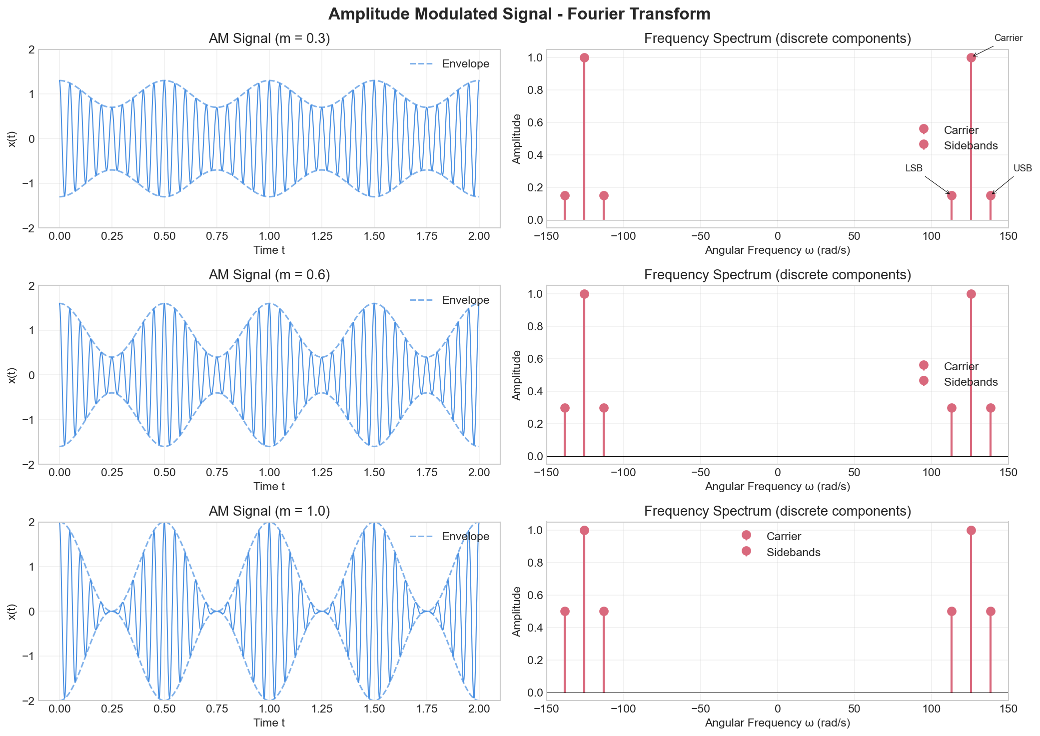
The figure shows AM signals with different modulation indices (m = 0.3, 0.6, 1.0). The time domain shows the characteristic amplitude variation following the message signal envelope. The frequency domain shows the three-component spectrum: a strong carrier component at ω_c and two sidebands at ω_c ± ω_m. As the modulation index increases, the sideband amplitudes grow relative to the carrier, carrying more information. The bandwidth is always 2ω_m regardless of the modulation index.

Example 5: Frequency Modulated (FM) Signal

Consider a frequency modulated signal:

$$x(t)=A\cos ({\omega }_{c}t+\beta \sin ({\omega }_{m}t))$$

where:

• $A$ is the carrier amplitude
• ${\omega }_c$ is the carrier frequency
• $\beta$ is the modulation index (frequency deviation ratio)
• ${\omega }_m$ is the message frequency

Using the Jacobi-Anger expansion, the FM signal can be expressed exactly as:

$$x(t)=A\cos ({\omega }_{c}t+\beta \sin ({\omega }_{m}t))=A\sum _{n=-\mathrm{\infty }}^{+\mathrm{\infty }}{J}_n(\beta )\cos (({\omega }_c+n{\omega }_m)t)$$

where $J_n(\beta )$ is the Bessel function of the first kind of order $n$.

The Fourier transform is:

$$X(\omega )=A\pi \sum _{n=-\mathrm{\infty }}^{+\mathrm{\infty }}{J}_n(\beta )[\delta (\omega -({\omega }_c+n{\omega }_m))+\delta (\omega +({\omega }_c+n{\omega }_m))]$$

Properties of Bessel functions:

• $J_{-n}(\beta )=(-1{)}^n{J}_n(\beta )$ (for integer $n$)
• $\sum _{n=-\mathrm{\infty }}^{+\mathrm{\infty }}{J}_n^2(\beta )=1$ (power conservation)
• For small $\beta$: $J_0(\beta )\approx 1$, $J_1(\beta )\approx \beta /2$, $J_n(\beta )\approx 0$ for $n\ge 2$
• For large $\beta$: significant sidebands up to $n\approx \beta +1$

Demonstration

The exact expansion using the Jacobi-Anger identity:

$$e^{j\beta \sin (\theta )}=\sum _{n=-\mathrm{\infty }}^{+\mathrm{\infty }}{J}_n(\beta )e^{jn\theta }$$

Applying this to the FM signal:

$$x(t)=A\text{Re}\{e^{j({\omega }_{c}t+\beta \sin ({\omega }_{m}t))}\}$$$$=A\text{Re}\{e^{j{\omega }_{c}t}{e}^{j\beta \sin ({\omega }_{m}t)}\}$$$$=A\text{Re}\{e^{j{\omega }_{c}t}\sum _{n=-\mathrm{\infty }}^{+\mathrm{\infty }}{J}_n(\beta )e^{jn{\omega }_{m}t}\}$$$$=A\sum _{n=-\mathrm{\infty }}^{+\mathrm{\infty }}{J}_n(\beta )\cos (({\omega }_c+n{\omega }_m)t)$$

Each term $J_n(\beta )\cos (({\omega }_c+n{\omega }_m)t)$ contributes a pair of impulses in the frequency domain at $\pm ({\omega }_c+n{\omega }_m)$, leading to the Fourier transform expression above.

Key observations:

• Narrowband FM: Similar spectrum to AM (carrier + 2 sidebands), but with phase relationships
• Wideband FM: Multiple sidebands at ${\omega }_c\pm n{\omega }_m$, amplitudes decay according to Bessel functions
• Bandwidth (Carson's rule): $BW\approx 2(\beta +1){\omega }_m$
• Larger $\beta$ → wider bandwidth but better noise immunity
• FM provides better signal-to-noise ratio than AM

Visualization:

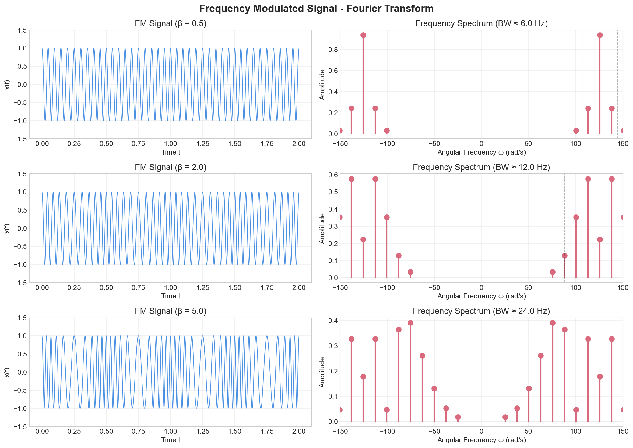
The figure shows FM signals with different modulation indices (β = 0.5, 2.0, 5.0). For narrowband FM (β = 0.5), the spectrum is similar to AM with a carrier and two sidebands. As β increases (wideband FM), multiple sidebands appear at ω_c ± nω_m, with amplitudes following Bessel function profiles. The bandwidth increases with β according to Carson's rule: BW ≈ 2(β + 1)ω_m. This demonstrates the frequency-domain trade-off in FM: wider bandwidth provides better noise immunity.