Chapter 3: Fourier Series

Introduction

The Fourier series represents periodic signals as a sum of harmonically related sinusoids or complex exponentials.

Periodic Signals

Definition: Periodic Signal

A signal $x(t)$ is periodic with period $T_0$ if:

$$x(t+T_0)=x(t)\text{for all }t$$

The fundamental frequency is $f_0=1/T_0$ and the fundamental angular frequency is ${\omega }_0=2\pi /T_0$.

Complex Exponential Fourier Series

Theorem: Fourier Series Representation

A periodic signal $x(t)$ with period $T_0$ can be represented as:

$$x(t)=\sum _{k=-\mathrm{\infty }}^{+\mathrm{\infty }}{c}_k{e}^{jk{\omega }_{0}t}$$

where the Fourier coefficients are:

$$c_k=\frac{1}{T_0}{\int }_{T_0}x(t)e^{-jk{\omega }_{0}t}dt$$

Properties of Fourier Coefficients

Proposition: Symmetry Properties

For a real signal $x(t)$:

• $c_{-k}=c_k^{\ast }$ (conjugate symmetry)
• $|c_{-k}|=|c_k|$ (even magnitude spectrum)
• $\mathrm{\angle }{c}_{-k}=-\mathrm{\angle }{c}_k$ (odd phase spectrum)

Representation: Line Spectra

The Fourier series representation can be visualized using line spectra, which show the magnitude and phase of each harmonic component.

Definition: Line Spectra

For a periodic signal with Fourier coefficients $c_k$, we define:

1. Magnitude Spectrum (or Amplitude Spectrum): A plot of $|c_k|$ versus $k$
2. Phase Spectrum: A plot of $\mathrm{\angle }{c}_k$ versus $k$

The line spectra are discrete, with non-zero values only at integer multiples of the fundamental frequency ${\omega }_0$.

Properties:

For real signals $x(t)$:

• The magnitude spectrum is even: $|c_{-k}|=|c_k|$
• The phase spectrum is odd: $\mathrm{\angle }{c}_{-k}=-\mathrm{\angle }{c}_k$
• Only the positive frequencies (k ≥ 0) need to be displayed due to symmetry

Interpretation:

• Each line at frequency $k{\omega }_0$ represents a harmonic component
• The height of each line indicates the amplitude of that harmonic
• The DC component $c_0$ represents the average value of the signal
• Higher harmonics contribute to the fine details and sharp transitions in the signal
• The rate of decay of $|c_k|$ as $k\to \mathrm{\infty }$ indicates the smoothness of the signal:
  • Discontinuities → slow decay (e.g., $|c_k|\sim 1/k$)
  • Continuous but non-smooth → faster decay (e.g., $|c_k|\sim 1/k^2$)
  • Smooth signals → rapid decay (e.g., exponential)

Example Visualization:

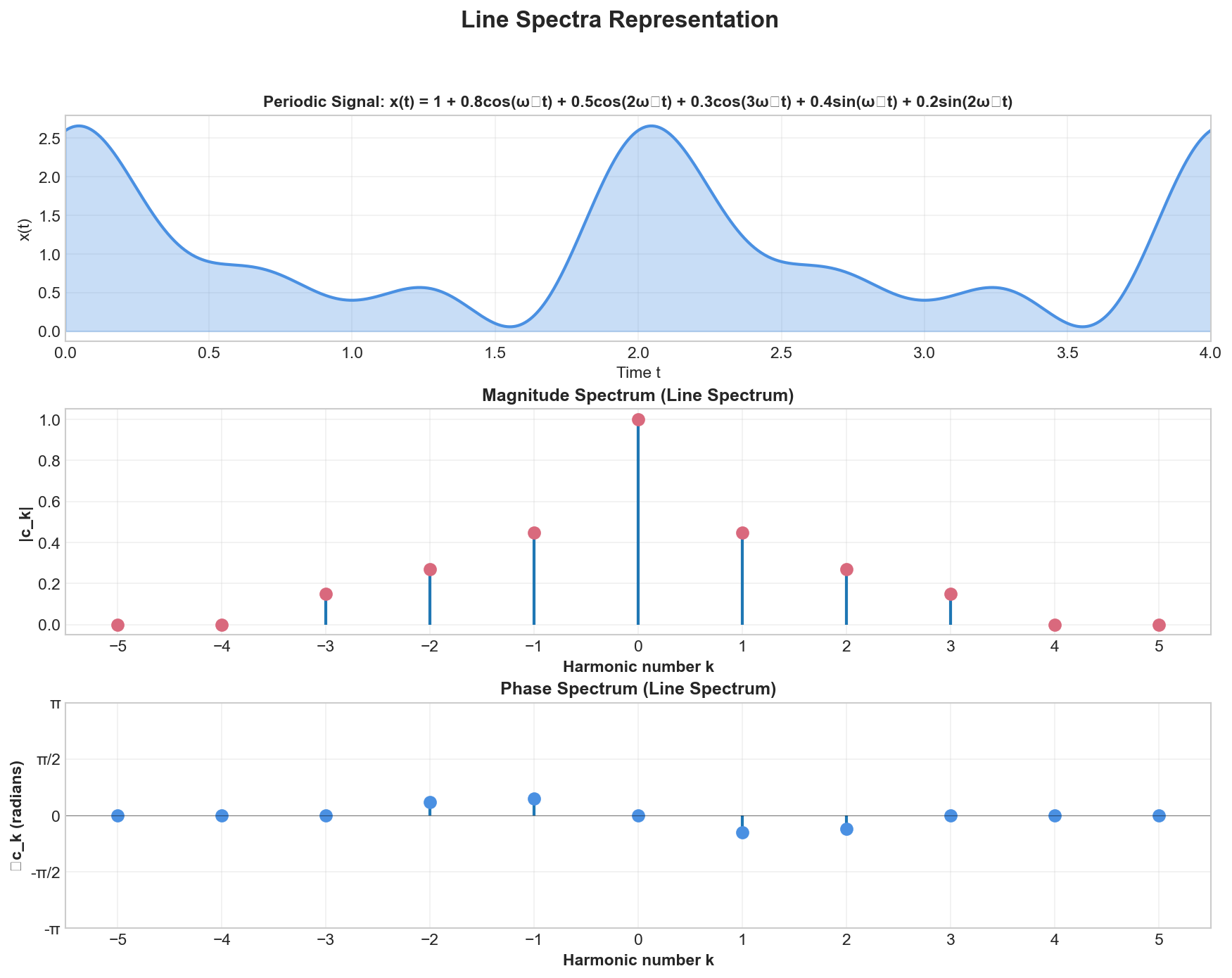
The figure illustrates line spectra for a periodic signal composed of a DC component and three harmonics. The magnitude spectrum (middle) shows the even symmetry property: $|c_{-k}|=|c_k|$. The phase spectrum (bottom) shows the odd symmetry property: $\mathrm{\angle }{c}_{-k}=-\mathrm{\angle }{c}_k$. The DC component at k = 0 represents the average value of the signal. Notice that the spectrum is discrete, with non-zero values only at integer multiples of the fundamental frequency.

Trigonometric Fourier Series

Definition: Trigonometric Form

For real signals, the Fourier series can be written as:

$$x(t)=a_0+\sum _{k=1}^{\mathrm{\infty }}[a_k\cos (k{\omega }_{0}t)+b_k\sin (k{\omega }_{0}t)]$$

where:

$$a_0=\frac{1}{T_0}{\int }_{T_0}x(t)dt$$$$a_k=\frac{2}{T_0}{\int }_{T_0}x(t)\cos (k{\omega }_{0}t)dt$$$$b_k=\frac{2}{T_0}{\int }_{T_0}x(t)\sin (k{\omega }_{0}t)dt$$

Relationship Between Forms

$$c_0=a_0,c_k=\frac{a_k-j{b}_k}{2},c_{-k}=\frac{a_k+j{b}_k}{2}$$

Parseval's Theorem

Theorem: Parseval's Theorem for Fourier Series

The average power of a periodic signal equals the sum of powers in each harmonic:

$$P=\frac{1}{T_0}{\int }_{T_0}|x(t){|}^{2}dt=\sum _{k=-\mathrm{\infty }}^{+\mathrm{\infty }}|c_k{|}^2$$

Properties of Fourier Series

Property	Time Domain	Frequency Domain
Linearity	$ax(t)+by(t)$	$a{c}_k^{(x)}+b{c}_k^{(y)}$
Time Shift	$x(t-t_0)$	$c_k{e}^{-jk{\omega }_0{t}_0}$
Frequency Shift	$x(t)e^{jm{\omega }_{0}t}$	$c_{k-m}$
Time Reversal	$x(-t)$	$c_{-k}$
Differentiation	$\frac{dx(t)}{dt}$	$jk{\omega }_0{c}_k$
Convolution	$x(t)\ast y(t)$	$T_0{c}_k^{(x)}{c}_k^{(y)}$

Convergence

Definition: Dirichlet Conditions

A periodic signal $x(t)$ has a convergent Fourier series if:

1. $x(t)$ is absolutely integrable over one period
2. $x(t)$ has a finite number of maxima and minima in one period
3. $x(t)$ has a finite number of discontinuities in one period

Examples

Example 1: Square Wave

Consider a square wave with amplitude $A$ and period $T_0$:

$$x(t)=\{\begin{array}{ll}A& ,0<t<T_0/2\\ -A& ,T_0/2<t<T_0\end{array}$$

The Fourier coefficients are given by :

$$c_k=\{\begin{array}{ll}0& k\text{ even}\\ \frac{2A}{jk\pi }& k\text{ odd}\end{array}$$

This gives the series:

$$x(t)=\frac{4A}{\pi }[\sin ({\omega }_{0}t)+\frac{1}{3}\sin (3{\omega }_{0}t)+\frac{1}{5}\sin (5{\omega }_{0}t)+\cdots ]$$

Demonstration

Computing the Fourier coefficients:

We compute $c_k=\frac{1}{T_0}{\int }_0^{T_0}x(t)e^{-jk{\omega }_{0}t}dt$.

For $k=0$:

$$c_0=\frac{1}{T_0}[{\int }_0^{T_0/2}Adt+{\int }_{T_0/2}^{T_0}(-A)dt]=\frac{1}{T_0}[\frac{A{T}_0}{2}-\frac{A{T}_0}{2}]=0$$

For $k\ne 0$, split the integral:

$$c_k=\frac{1}{T_0}[A{\int }_0^{T_0/2}{e}^{-jk{\omega }_{0}t}dt-A{\int }_{T_0/2}^{T_0}{e}^{-jk{\omega }_{0}t}dt]$$

Evaluate each integral using $\int e^{-jk{\omega }_{0}t}dt=\frac{e^{-jk{\omega }_{0}t}}{-jk{\omega }_0}$:

$${\int }_0^{T_0/2}{e}^{-jk{\omega }_{0}t}dt=\frac{1}{-jk{\omega }_0}[e^{-jk{\omega }_0{T}_0/2}-1]=\frac{1}{jk{\omega }_0}[1-e^{-jk\pi }]$$$${\int }_{T_0/2}^{T_0}{e}^{-jk{\omega }_{0}t}dt=\frac{1}{-jk{\omega }_0}[e^{-jk{\omega }_0{T}_0}-e^{-jk{\omega }_0{T}_0/2}]=\frac{1}{jk{\omega }_0}[e^{-jk\pi }-1]$$

where we used ${\omega }_0{T}_0=2\pi$ and $e^{-j2\pi k}=1$.

Substituting back:

$$c_k=\frac{A}{T_0}\cdot \frac{1}{jk{\omega }_0}[1-e^{-jk\pi }-e^{-jk\pi }+1]=\frac{2A}{jk{\omega }_0{T}_0}(1-e^{-jk\pi })$$

Since ${\omega }_0{T}_0=2\pi$:

$$c_k=\frac{A}{jk\pi }(1-e^{-jk\pi })$$

Now, $e^{-jk\pi }=\cos (k\pi )=(-1{)}^k$ (since $\sin (k\pi )=0$), therefore:

$$1-e^{-jk\pi }=1-(-1{)}^k=\{\begin{array}{ll}0& k\text{ even}\\ 2& k\text{ odd}\end{array}$$

Thus:

$$c_k=\{\begin{array}{ll}0& k\text{ even or }k=0\\ \frac{2A}{jk\pi }& k\text{ odd}\end{array}$$

Deriving the trigonometric series:

For odd $k$, we have $c_k=\frac{2A}{jk\pi }=-j\frac{2A}{k\pi }$ and by conjugate symmetry, $c_{-k}=j\frac{2A}{k\pi }$.

The contribution from harmonics $\pm k$ is:

$$c_k{e}^{jk{\omega }_{0}t}+c_{-k}{e}^{-jk{\omega }_{0}t}=-j\frac{2A}{k\pi }{e}^{jk{\omega }_{0}t}+j\frac{2A}{k\pi }{e}^{-jk{\omega }_{0}t}$$$$=j\frac{2A}{k\pi }(e^{-jk{\omega }_{0}t}-e^{jk{\omega }_{0}t})=j\frac{2A}{k\pi }\cdot (-2j\sin (k{\omega }_{0}t))=\frac{4A}{k\pi }\sin (k{\omega }_{0}t)$$

Summing over odd $k=1,3,5,\dots$ gives:

$$x(t)=\frac{4A}{\pi }[\sin ({\omega }_{0}t)+\frac{1}{3}\sin (3{\omega }_{0}t)+\frac{1}{5}\sin (5{\omega }_{0}t)+\cdots ]$$

Visualization:

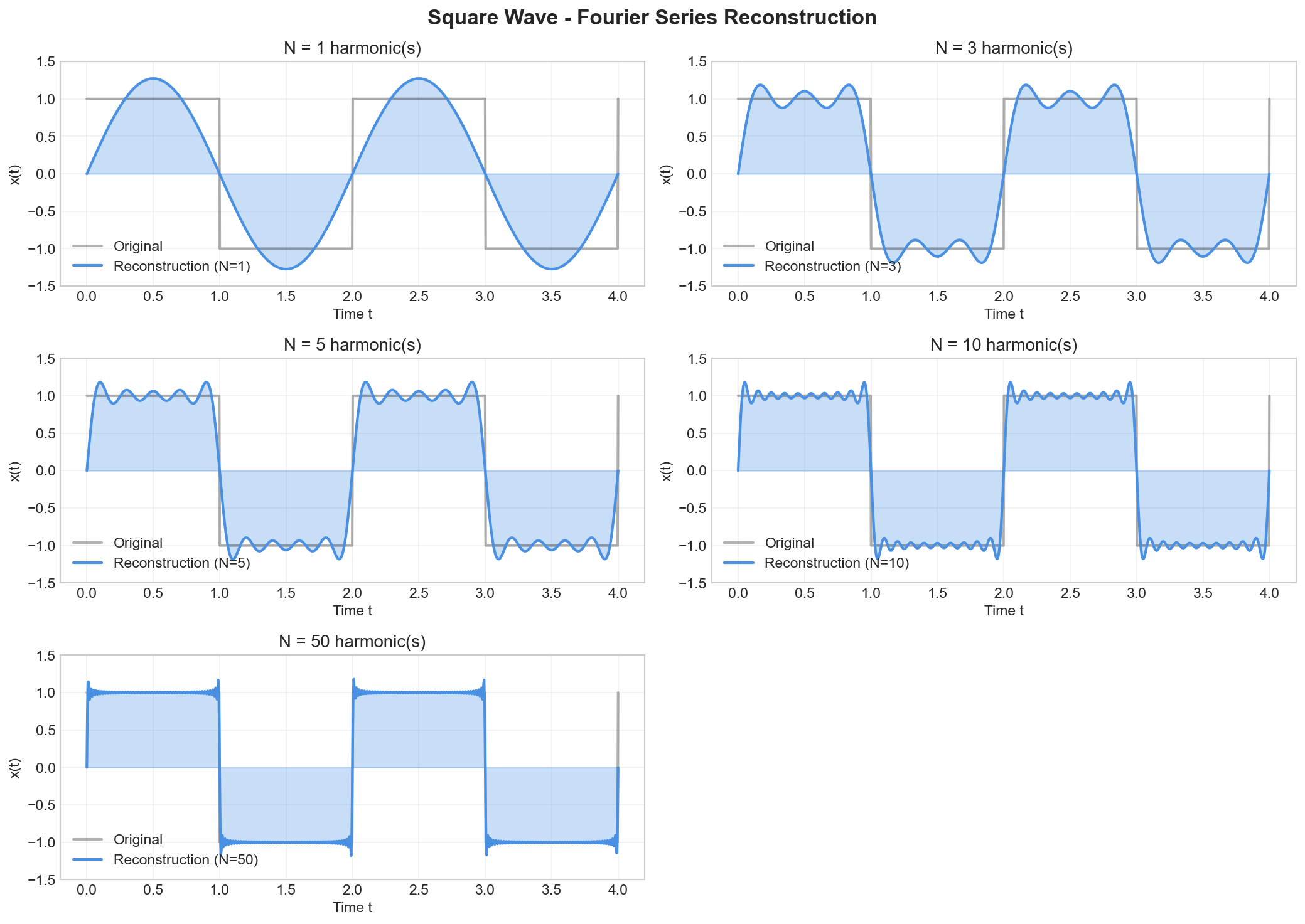
The figure above shows how the Fourier series approximation improves as more harmonics are added. Notice the Gibbs phenomenon at the discontinuities - the overshoots persist even with many harmonics.

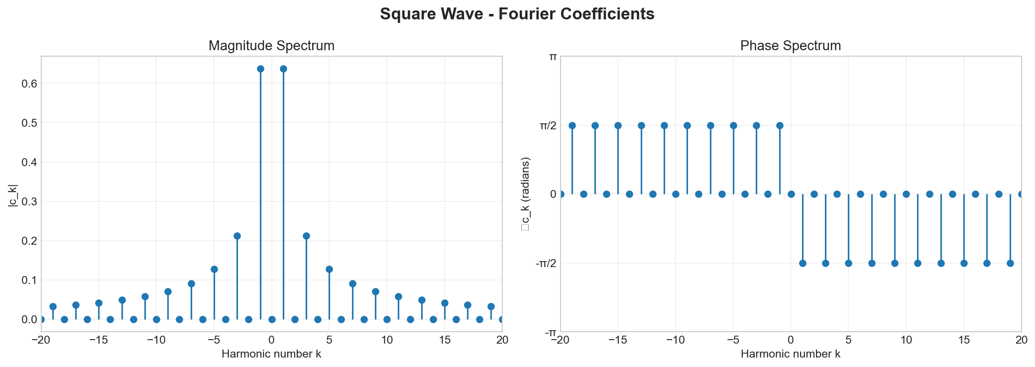
The magnitude spectrum shows that only odd harmonics are present, with magnitude decaying as 1/k. The phase spectrum shows that all coefficients have phase ±π/2.

Example 2: Sawtooth Wave

Consider a sawtooth wave increasing linearly from $-A$ to $A$ over one period $T_0$, centered at $t=0$:

$$x(t)=\frac{2A}{T_0}t,-\frac{T_0}{2}<t<\frac{T_0}{2}$$

The Fourier coefficients are given by :

$$c_k=\frac{1}{T_0}{\int }_0^{T_0}x(t)e^{-jk{\omega }_{0}t}dt$$

This gives the series:

$$x(t)=\frac{2A}{\pi }\sum _{k=1}^{\mathrm{\infty }}\frac{(-1{)}^{k+1}}{k}\sin (k{\omega }_{0}t)$$

Demonstration

Computing the Fourier coefficients:

We have $x(t)=\frac{2A}{T_0}t$ for $-\frac{T_0}{2}<t<\frac{T_0}{2}$.

Observation: Since $x(t)$ is an odd function ($x(-t)=-x(t)$), we expect $c_k$ to be purely imaginary.

For $k=0$:

$$c_0=\frac{1}{T_0}{\int }_{-T_0/2}^{T_0/2}\frac{2A}{T_0}tdt=\frac{2A}{T_0^2}{\left[\frac{t^2}{2}\right]}_{-T_0/2}^{T_0/2}=\frac{A}{T_0^2}[\frac{T_0^2}{4}-\frac{T_0^2}{4}]=0$$

For $k\ne 0$:

$$c_k=\frac{1}{T_0}{\int }_{-T_0/2}^{T_0/2}\frac{2A}{T_0}t\cdot e^{-jk{\omega }_{0}t}dt=\frac{2A}{T_0^2}{\int }_{-T_0/2}^{T_0/2}t\cdot e^{-jk{\omega }_{0}t}dt$$

Use integration by parts with $u=t$ and $dv=e^{-jk{\omega }_{0}t}dt$:

$${\int }_{-T_0/2}^{T_0/2}t\cdot e^{-jk{\omega }_{0}t}dt={\left[\frac{t\cdot e^{-jk{\omega }_{0}t}}{-jk{\omega }_0}\right]}_{-T_0/2}^{T_0/2}-{\int }_{-T_0/2}^{T_0/2}\frac{e^{-jk{\omega }_{0}t}}{-jk{\omega }_0}dt$$

Evaluating the first term:

$${\left[\frac{t\cdot e^{-jk{\omega }_{0}t}}{-jk{\omega }_0}\right]}_{-T_0/2}^{T_0/2}=\frac{T_0/2\cdot e^{-jk\pi }}{-jk{\omega }_0}-\frac{(-T_0/2)\cdot e^{jk\pi }}{-jk{\omega }_0}$$

Since $e^{jk\pi }=e^{-jk\pi }=(-1{)}^k$:

$$=\frac{(-1{)}^k}{-jk{\omega }_0}(\frac{T_0}{2}+\frac{T_0}{2})=\frac{(-1{)}^k{T}_0}{-jk{\omega }_0}$$

Evaluating the second term:

$${\int }_{-T_0/2}^{T_0/2}\frac{e^{-jk{\omega }_{0}t}}{-jk{\omega }_0}dt=\frac{1}{-jk{\omega }_0}{\left[\frac{e^{-jk{\omega }_{0}t}}{-jk{\omega }_0}\right]}_{-T_0/2}^{T_0/2}=\frac{1}{(jk{\omega }_0{)}^2}[e^{-jk\pi }-e^{jk\pi }]=0$$

(since $e^{-jk\pi }=e^{jk\pi }=(-1{)}^k$).

Therefore:

$$c_k=\frac{2A}{T_0^2}\cdot \frac{(-1{)}^k{T}_0}{-jk{\omega }_0}=\frac{2A(-1{)}^k}{-jk{\omega }_0{T}_0}$$

Since ${\omega }_0{T}_0=2\pi$:

$$c_k=\frac{A(-1{)}^k}{-jk\pi }=\frac{A(-1{)}^{k+1}}{jk\pi }$$

Deriving the trigonometric series:

For the real signal with odd symmetry, we have $c_k=\frac{A(-1{)}^{k+1}}{jk\pi }$ (purely imaginary).

By conjugate symmetry, $c_{-k}=c_k^{\ast }=\frac{A(-1{)}^{k+1}}{-jk\pi }$.

The contribution from harmonics $\pm k$ is:

$$c_k{e}^{jk{\omega }_{0}t}+c_{-k}{e}^{-jk{\omega }_{0}t}=\frac{A(-1{)}^{k+1}}{jk\pi }{e}^{jk{\omega }_{0}t}-\frac{A(-1{)}^{k+1}}{jk\pi }{e}^{-jk{\omega }_{0}t}$$$$=\frac{A(-1{)}^{k+1}}{jk\pi }(e^{jk{\omega }_{0}t}-e^{-jk{\omega }_{0}t})=\frac{A(-1{)}^{k+1}}{jk\pi }\cdot 2j\sin (k{\omega }_{0}t)=\frac{2A(-1{)}^{k+1}}{k\pi }\sin (k{\omega }_{0}t)$$

Summing over all $k=1,2,3,\dots$ gives:

$$x(t)=\frac{2A}{\pi }\sum _{k=1}^{\mathrm{\infty }}\frac{(-1{)}^{k+1}}{k}\sin (k{\omega }_{0}t)$$$$=\frac{2A}{\pi }[\sin ({\omega }_{0}t)-\frac{1}{2}\sin (2{\omega }_{0}t)+\frac{1}{3}\sin (3{\omega }_{0}t)-\frac{1}{4}\sin (4{\omega }_{0}t)+\cdots ]$$

Visualization:

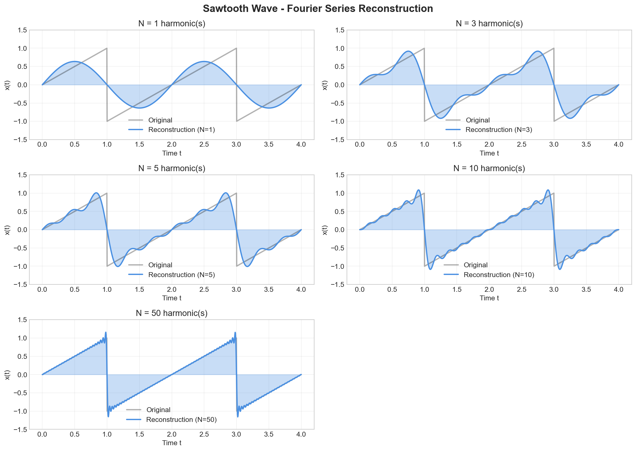
The figure shows the Fourier series reconstruction of the sawtooth wave. The convergence is smoother compared to the square wave since the sawtooth has no discontinuities, only a discontinuity in the derivative.

The magnitude spectrum shows all harmonics (both even and odd) are present, decaying as 1/k. The phase spectrum shows alternating phases of ±π/2, corresponding to the alternating sign in the series coefficients.

Example 3: Pulse train with duty cycle $\alpha$

Consider a periodic pulse train of period $T_0$, amplitude $A$, and duty cycle ($0<\alpha <1$):

$$x(t)=\{\begin{array}{ll}A& 0<t<\alpha T_0\\ 0& \alpha T_0<t<T_0\end{array}$$

The Fourier coefficients are given by :

$$c_k=\{\begin{array}{ll}\frac{A}{jk2\pi }(1-e^{-jk2\pi \alpha })& ,k\ne 0\\ A\alpha & ,k=0\end{array}$$

Thus the complex Fourier series:

$$x(t)=A\alpha +\sum _{k\ne 0}\frac{A}{jk2\pi }(1-e^{-jk2\pi \alpha })e^{jk{\omega }_{0}t}$$

Demonstration

Computing the Fourier coefficients:

We compute $c_k=\frac{1}{T_0}{\int }_0^{T_0}x(t)e^{-jk{\omega }_{0}t}dt$.

For $k=0$:

$$c_0=\frac{1}{T_0}{\int }_0^{\alpha T_0}Adt=\frac{A}{T_0}\cdot \alpha T_0=A\alpha$$

This is the DC component (average value) of the signal.

For $k\ne 0$:

$$c_k=\frac{1}{T_0}{\int }_0^{\alpha T_0}A{e}^{-jk{\omega }_{0}t}dt=\frac{A}{T_0}{\int }_0^{\alpha T_0}{e}^{-jk{\omega }_{0}t}dt$$

Evaluate the integral:

$${\int }_0^{\alpha T_0}{e}^{-jk{\omega }_{0}t}dt={\left[\frac{e^{-jk{\omega }_{0}t}}{-jk{\omega }_0}\right]}_0^{\alpha T_0}=\frac{1}{-jk{\omega }_0}(e^{-jk{\omega }_0\alpha T_0}-1)$$$$=\frac{1}{jk{\omega }_0}(1-e^{-jk{\omega }_0\alpha T_0})$$

Since ${\omega }_0{T}_0=2\pi$, we have $k{\omega }_0\alpha T_0=k\cdot 2\pi \alpha$:

$$c_k=\frac{A}{T_0}\cdot \frac{1}{jk{\omega }_0}(1-e^{-jk2\pi \alpha })=\frac{A}{jk{\omega }_0{T}_0}(1-e^{-jk2\pi \alpha })$$

Since ${\omega }_0{T}_0=2\pi$:

$$c_k=\frac{A}{jk2\pi }(1-e^{-jk2\pi \alpha })$$

Alternative form using the sinc function:

We can rewrite the coefficient using Euler's formula. Note that:

$$1-e^{-jk2\pi \alpha }=1-\cos (k2\pi \alpha )+j\sin (k2\pi \alpha )$$

We can also express this as:

$$c_k=\frac{A}{jk2\pi }\cdot 2e^{-jk\pi \alpha }(e^{jk\pi \alpha }-e^{-jk\pi \alpha })/2=\frac{A\alpha }{k\pi \alpha }{e}^{-jk\pi \alpha }\sin (k\pi \alpha )$$$$=A\alpha \cdot \text{sinc}(k\alpha )\cdot e^{-jk\pi \alpha }$$

where $\text{sinc}(x)=\frac{\sin (\pi x)}{\pi x}$.

Summary of results:

$$c_k=\{\begin{array}{ll}A\alpha & k=0\\ \frac{A}{jk2\pi }(1-e^{-jk2\pi \alpha })& k\ne 0\end{array}$$

The complex Fourier series is:

$$x(t)=A\alpha +\sum _{k\ne 0}\frac{A}{jk2\pi }(1-e^{-jk2\pi \alpha })e^{jk{\omega }_{0}t}$$

Visualization:

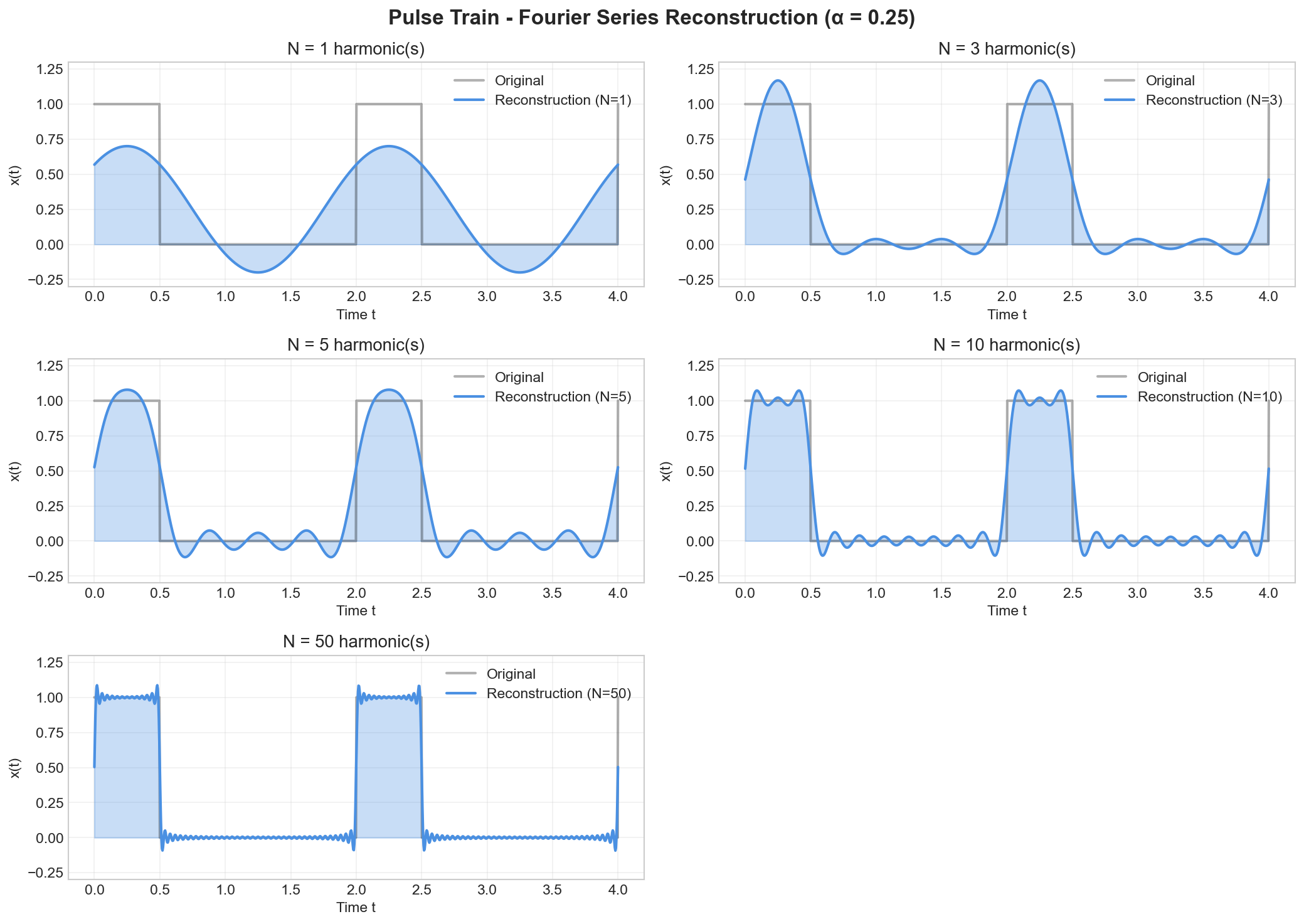
The figure shows the Fourier series reconstruction of a pulse train with 25% duty cycle (α = 0.25). As more harmonics are added, the reconstruction improves, with the Gibbs phenomenon visible at the discontinuities (similar to the square wave). The DC component c₀ = Aα = 0.25A gives the average value.

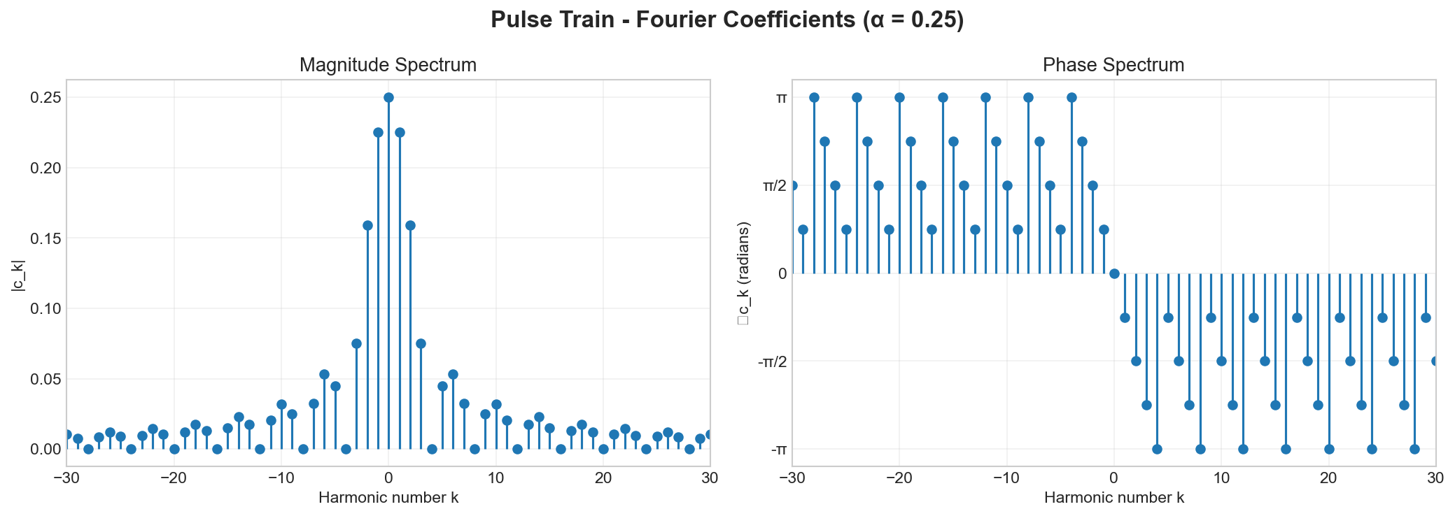
The magnitude and phase spectra for a 25% duty cycle pulse train. Notice that all harmonics are present (unlike the square wave which has only odd harmonics). The DC component c₀ = 0.25A is visible at k = 0. The narrow pulse (25% duty cycle) requires more harmonics for accurate reconstruction.

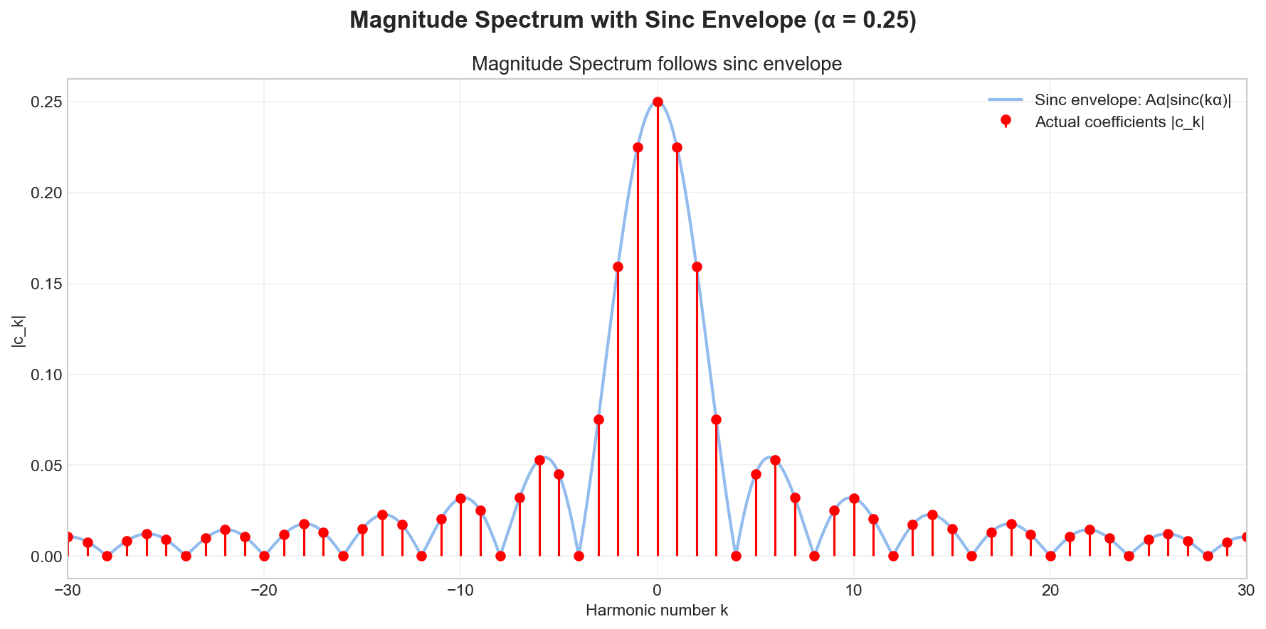
The magnitude spectrum follows a sinc envelope, as predicted by the analytical formula |c_k| = Aα|sinc(kα)|. The zeros of the sinc function occur at integer multiples of 1/α, which for α = 0.25 means zeros at k = ±4, ±8, ±12, etc. This is characteristic of rectangular pulses: narrower pulses (smaller α) have a wider sinc envelope, requiring more harmonics for accurate reconstruction.